This notebook is the first of a series of notebooks based on a talk I gave at the CUDAN 2023 conference in Tallinn, Estonia (https://cudan.tlu.ee/conference/) together with Melvin Wevers and Mike Kestemont, titled Steady Formulas, Shifting Spells: Estimating Folktale Diversity.
Comparing Cultural Diversity Estimates
Quantifying the diversity of cultural collections presents many unique challenges. In earlier posts (e.g., Demystifying Chao1 with Good-Turing and Population Size Estimation as a Regression Problem), I’ve discussed the issue of undersampling in cultural collections, largely as a consequence of cultural loss. In this post, I discuss some problems when comparing diversity measurements: When and how can we assert that one collection is more diverse than another?
The collection I study in this notebook is a unique assemblage of Dutch folktales, gathered by the Meertens Institute in the 1960s and 70s. Embarking on an ambitious project to create a comprehensive Dutch folktale atlas, the institute recruited a group of dedicated folktale collectors. These collectors were tasked with visiting storytellers within specific areas around their homes, ultimately with the aim of covering the entire map of the Netherlands. This groundbreaking endeavor in folklore research led to the collection of over 32,000 stories. However, as indicated by the map below, many regions of the Netherlands remained uncharted in this collection, highlighting gaps and the diverse interests of the collectors in shaping its completeness and reliability.
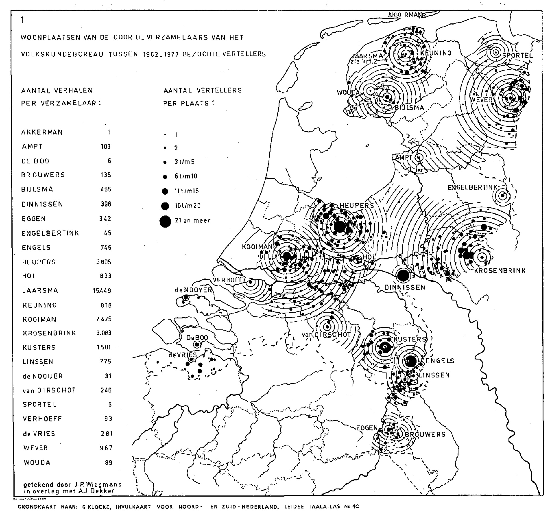
Figure 1: Map by A.J. Dekker showing the residences of the narrators visited by the collectors of the Folklore Bureau between 1962 and 1977.
Cultural diversity manifests in various forms, and one of the simplest methods to gauge the diversity in collections such as these folktales is by counting the unique items or unique categories within them. Referred to as the ‘richness’ of the collection, this metric offers a quick snapshot of their diversity. However, this simplicity comes with a downside. The richness measurement is notably sensitive; even minor changes in the collection can significantly impact the result. Furthermore, there is a strong correlation between the perceived richness and the size of the sample (Chao and Jost 2012). And this correlation can greatly impede comparisons across different collections.
This correlation is clearly present in the collection of folktales, where the sampling effort of the collectors varies greatly. Take the folktale collector Dam Jaarsma, for example. He compiled a collection with over 15 thousand stories. These stories can be classified into more than 600 unique folktale types (such as the ones by Uther 2004). By contrast, a collection of someone like Kooijman consists of a little over 2 thousand stories, which can be grouped into a little over 100 different types. Strictly speaking, the collection of Jaarsma is more diverse than that of Kooijman, yet intuitively it feels unfair to state that the area where these stories were sampled from are more or less diverse, as it so strongly depends on the collectors’ search efforts. This strong correlation between sample size and richness is further illustrated in the following plot:
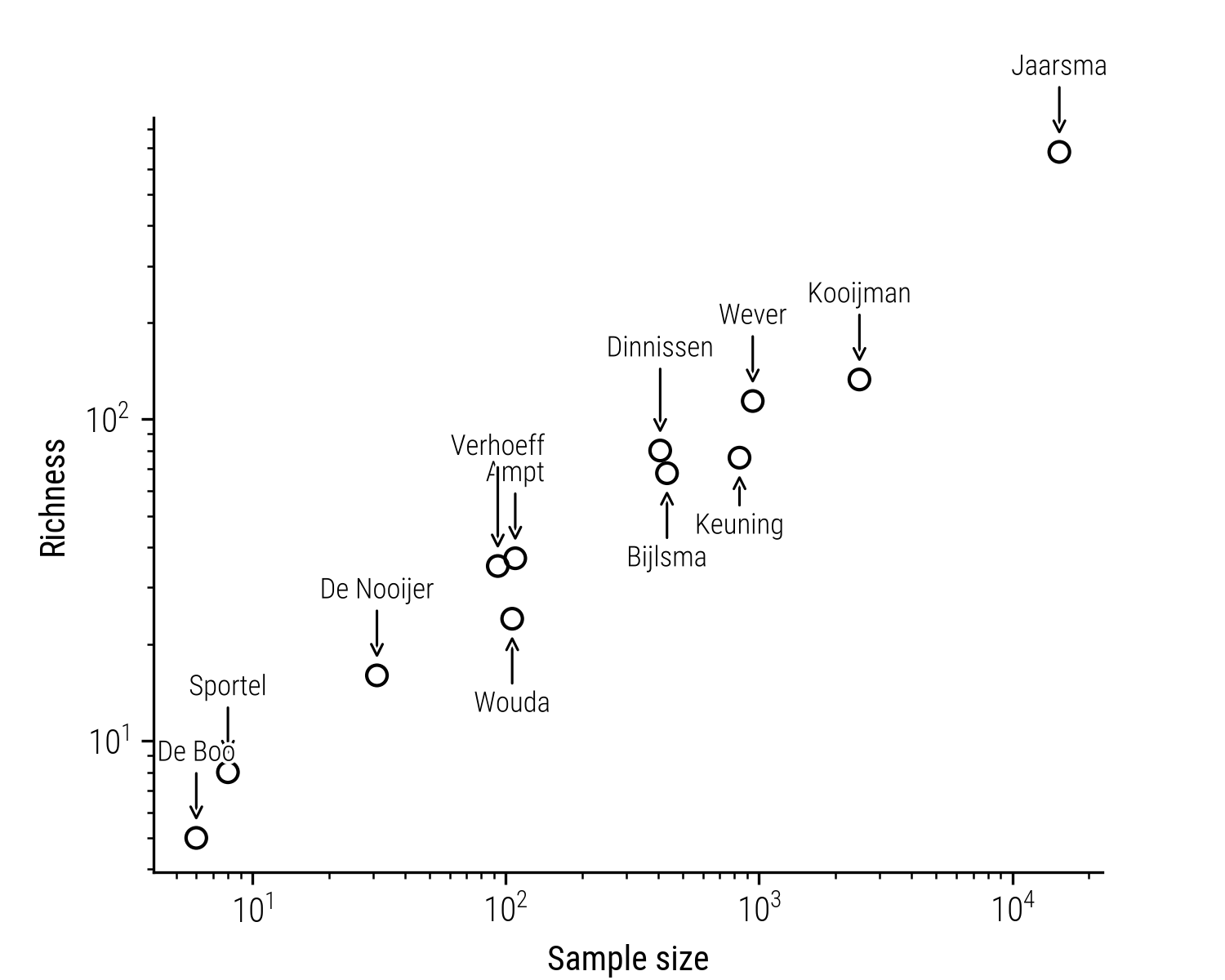
Figure 2: Relation between the sample size (measure in number of stories) and unique story types.
Rarifying Species
Ecologists face a similar problem when measuring biological diversity. To adjust for the impact of sample size, ecologists have developed a method called rarefaction. This technique involves downsizing larger collections to match the size of the smallest sample. The essence of rarefaction lies in its ability to compute the richness of species for a specific count of individual samples. This is done through the construction of what are known as rarefaction curves. These curves graph the relationship between the number of species identified and the number of samples collected. They can be considered the statistical expection of the corresponding collector’s curve (also called ‘accumulation curve’ or ‘species discovery curve’), which records the empirical number of species reveiled as we progress to sample more individuals. Consider the plot below, depicting both an accumulation curve and its corresponding rarefaction curve:
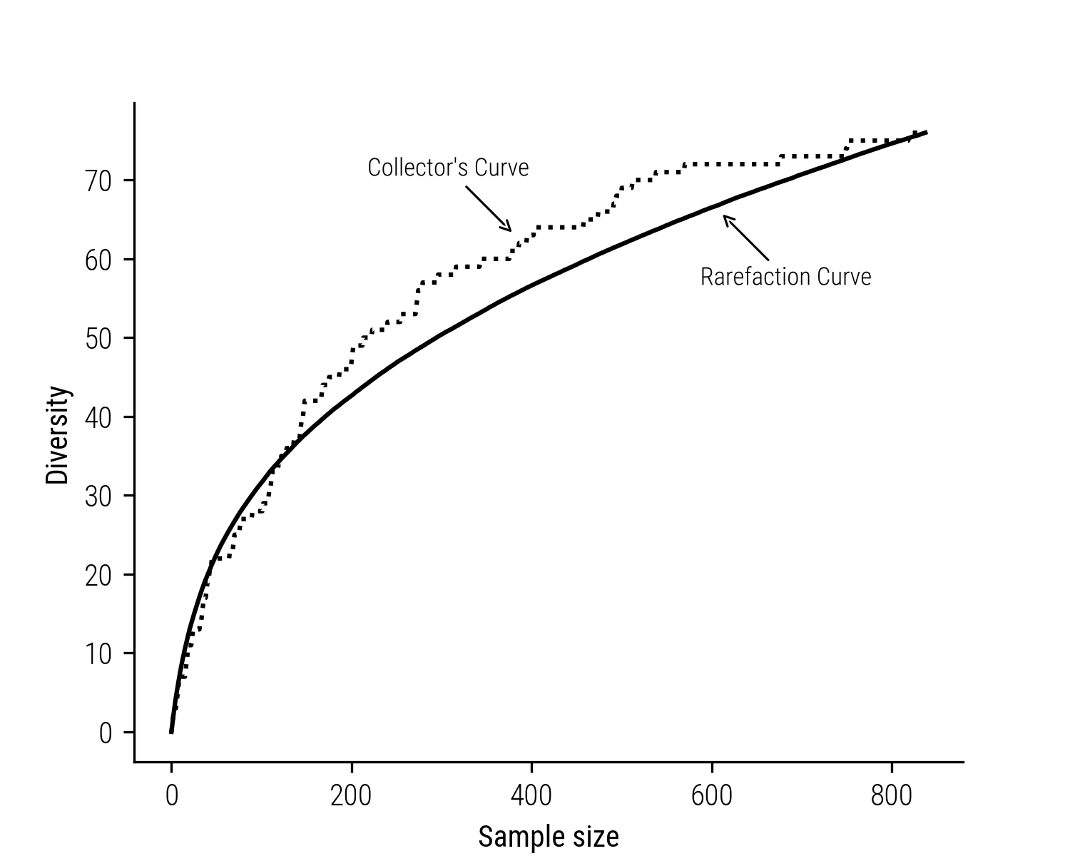
Figure 3: Fictional collector’s curve and its corresponding rarefaction curve.
Typically, these rarefaction curves rise quickly initially, capturing the most common species, and then level off as it becomes increasingly challenging to find new, rare species. The fundamental concept is that the more individuals you sample from a community, the more species you’re likely to encounter. To construct a rarefaction curve, ecologists repeatedly and randomly select subsets of size \(m\) from the total pool of \(N\) samples. They then plot the average species count found in each subset, ranging from 1 to \(N\). In essence, rarefaction predicts the expected species count in a smaller group of \(m\) individuals (or \(m\) samples), randomly selected from the larger set of \(N\) samples.
Rarifying Folktales
With this tool in hand, we can compare the richnesses folktale collections with different sample sizes, by standardizing the collections to the sample size of the smallest collection. For example, let’s compare the collections of Jaarsma and Keuning, who sampled 15,326 and 837 folktales respectively. We thus standardize the larger collection of Jaarsma to 837 stories and compute the rarefaction curve:
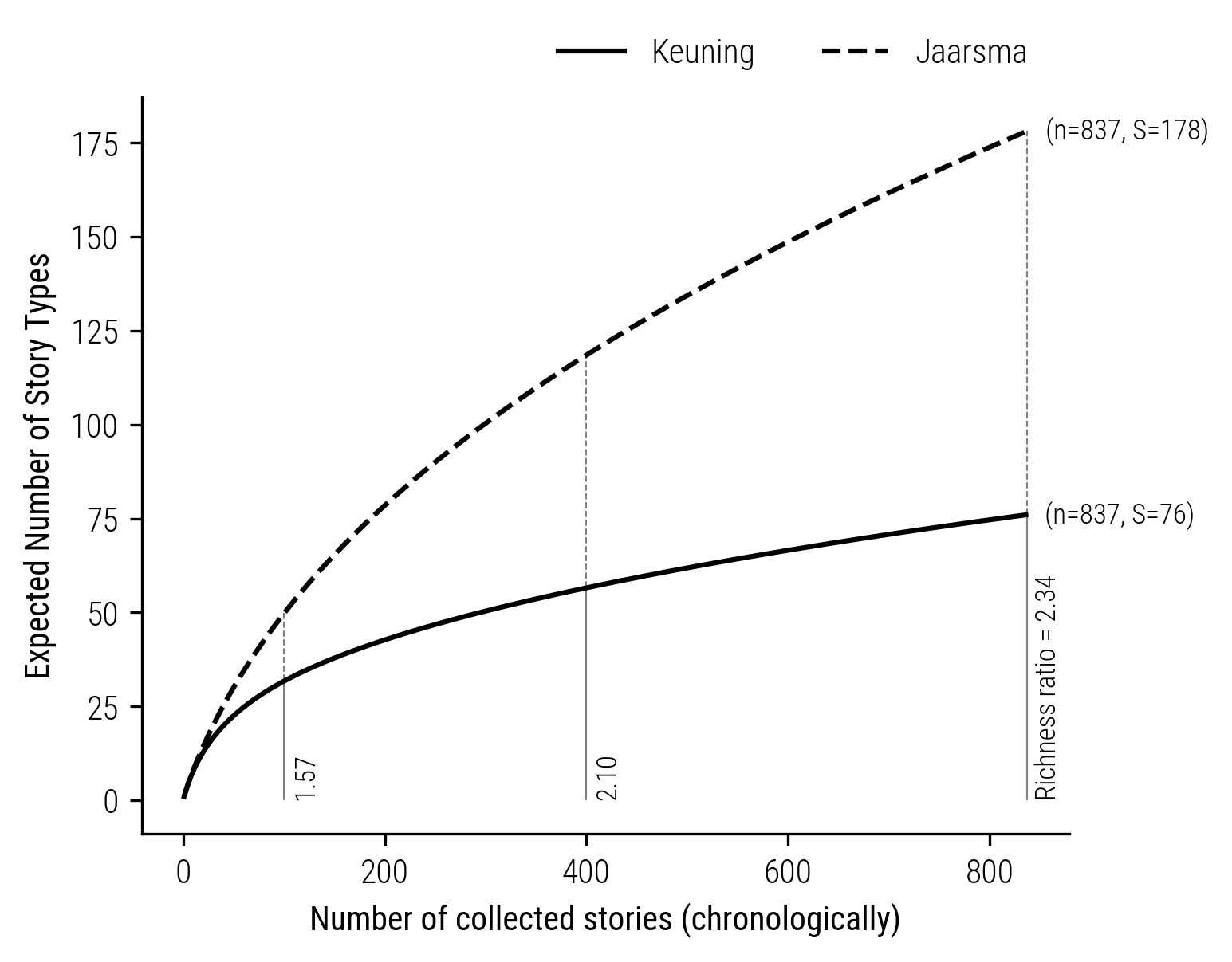
Figure 4: Comparison of Rarefaction curves of the collectors Jaarsma and Keuning.
This curve reveals the richness ratios between the two collections at various sample sizes. Starting from a ratio of 1.57 at a sample size of \(n=100\) and increasing to 2.34 at the complete collection of Keuning (\(n=837\)), it becomes evident that the apparent difference in richness is more a function of the chosen sample size rather than an intrinsic characteristic of the collections themselves. With higher degrees of rarification the underestimation of the degree of difference between the collections thus goes up.
Replication or Doubling Property
This phenomenon arises because estimating richness from samples of a fixed size fails to adhere to what is known as the ‘doubling property’ (Hill 1973) or ‘replication principle’ (Chao and Jost 2012). According to this principle, when two subsamples of equal size, each containing entirely distinct species but sharing the same abundance distribution, are combined, an desirable measure of diversity should reflect a doubling effect. The doubling principle is also what we intuitively expect from a diversity measure. If, for example, we study the richness of the combined sample, we would expect it to be twice as diverse (see Hill 1973 for a family of diversity measures that retain the doubling property even for higher order diversity values).
However, when estimating richness based on fixed sample sizes, as demonstrated in our rarefaction curves, the doubling property is not observed. To illustrate this, let’s consider an example from (Chao and Jost 2012), who examine two communities, \(A\) and \(B\). Each community has the same abundance distribution but no shared species:
A = np.arange(50)
pA = np.array([0.3] + [0.1] + [0.05] * 3 + [0.01] * 45)

B = np.arange(50, 100)
pB = pA.copy()
Suppose we sample 20 individuals (with replacement) from community \(A\). On average, this sample is expected to contain about 12 species:
n_iter = 1000
n_species = np.zeros(n_iter)

for i in range(n_iter):
    sample = np.random.choice(A, size=20, p=pA)
    n_species[i] = len(set(sample))
print(n_species.mean())
12.045
Now, consider a pooled sample from \(A+B\) and sample 20 individuals again. The expected number of species is not 24 (double of 12), but approximately 14:
n_iter = 1000
n_species = np.zeros(n_iter)

AB = np.hstack((A, B))
pAB = np.hstack((pA, pB))
pAB = pAB / pAB.sum()

for i in range(n_iter):
    sample = np.random.choice(AB, size=20, p=pAB)
    n_species[i] = len(set(sample))
print(n_species.mean())
14.274
These results indicate a significant underestimation of diversity. In this case, the richness difference ratio is approximately 1.18, far from the true value of 2. The rarefaction curve below highlights this discrepancy in further detail. It shows the instability of the richness ratio as a function of sample size and the absence of the doubling property, even at higher sample sizes.
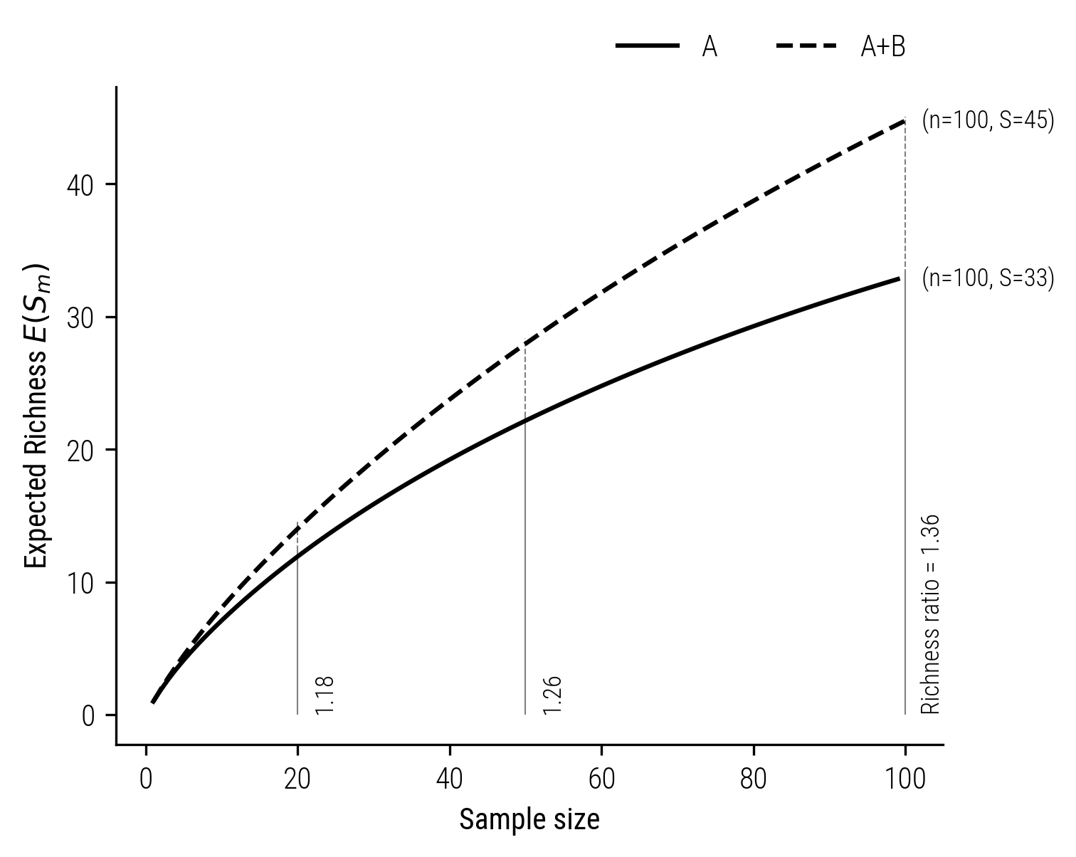
Figure 5: Rarefaction curve illustrating the absence of the doubling property when estimating richnesses based on samples of fixed size (based on Chao and Jost 2012)
Standardizing by Sample Coverage
As initially proposed by Alroy (2010) and further developed by Chao and Jost (2012), the key to addressing this issue lies in comparing samples based on equal completeness, or more precisely, equal coverage, rather than equal equal sample size. The term ‘coverage’ traces its roots back to the cryptographic work of Alan Turing during World War II. As Good highlighted in (1953), coverage is defined as the proportion of individuals in a community that are represented in a sample, belonging to the identified species. In simpler terms, it indicates the likelihood that a newly sampled individual will belong to a species already present in the sample.
Conversely, the term ‘coverage deficit’, as termed by Chao and colleagues in their (2012) paper, is calculated by subtracting the sample’s coverage from one. This deficit represents the portion of the community composed of species not yet included in the sample. Notably, the coverage deficit is a critical component in calculating the Unseen Species Estimator, known as Chao1 (Chao 1984). For a more detailed explanation, refer to my notebook ‘Demystifying Chao1 with Good-Turing’. The formula to estimate sample coverage is straightforward:
\begin{equation} \hat{C}_n = 1 - \frac{f_1}{n}, \end{equation}
where \(f_1\) is the count of species or categories that appear only once in the sample. An enhanced version of this estimator was proposed by Chao and Shen in 2010:
\begin{equation} \hat{C}_n = 1 - \frac{f_1}{n} \left [ \frac{(n - 1) f_1}{(n - 1) f_1 + 2 f_2} \right ] \end{equation}
As we will see, the key insight here is that when samples are standardized by coverage, the doubling property is approximately satisfied. And therefore, richness estimates of any two communities, when adjusted for coverage, provide a more accurate reflection of their actual diversity relationship, compared to traditional richness estimates based on fixed sample sizes. In the following plot, I compare the two communities \(A\) and \(A+B\) based on shared coverage values. The richness ratio satisfies the doubling principle, even for relatively small sample sizes and low coverage.
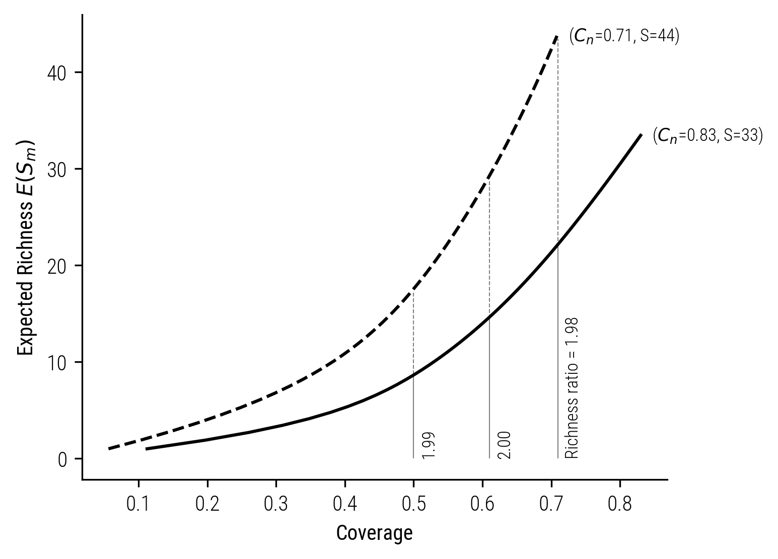
Figure 6: Illustration of Standardizing Rarefaction Curves by Coverage
Comparing Folktale Diversity by Coverage
This opens up quite exciting possibilities, as it would allow us to make meaningful judgements about about which community of cultural collection is more diverse than the other. This goes beyond simple rankings in terms of diversity. We’re now equipped to quantify the actual magnitude of these differences in diversity, as detailed by (/t Chao and Jost 2012). In the concluding part of this post, I will demonstrate the application of coverage-based rarefaction curves to the folktale collection compiled by the Meertens Institute.
We’ll start by comparing the collections of two folklorists, Jaarsma and Bijlsma, both of whom collected folktales in the Frysia province. The plot that follows illustrates the size-based rarefaction extrapolation curves for their respective collections.
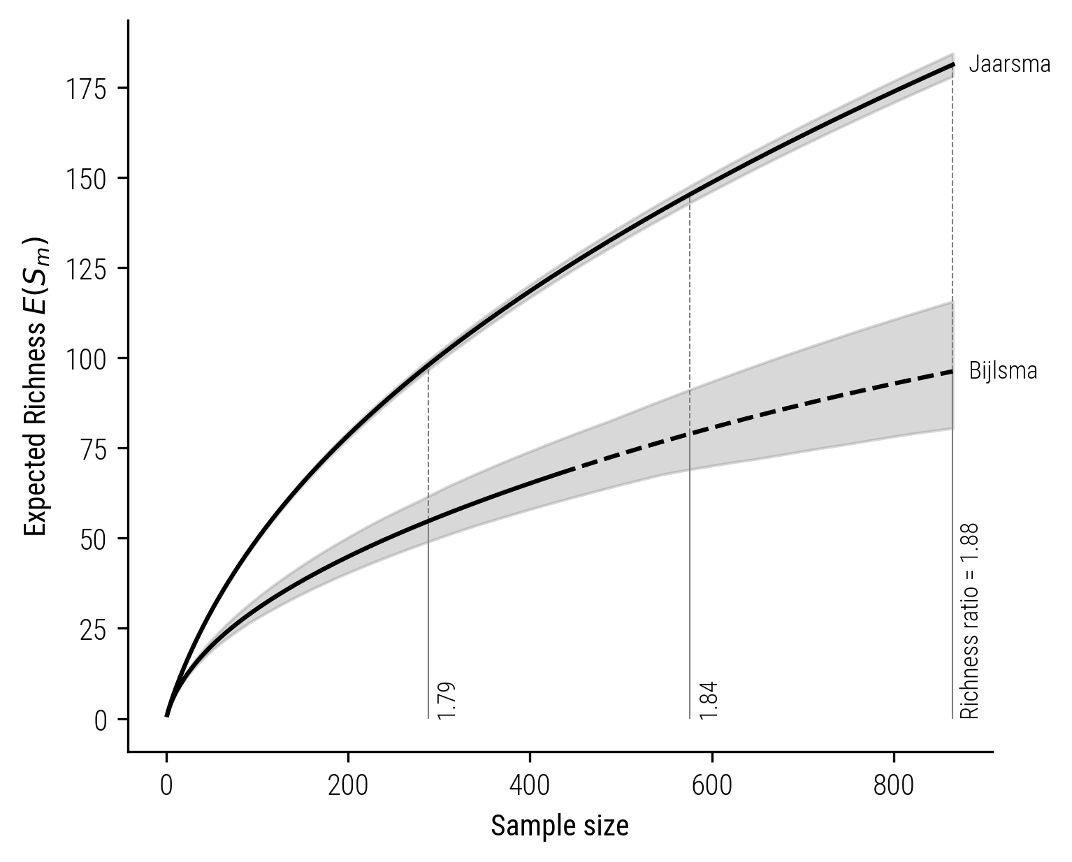
Figure 7: Size-based rarefaction-extrapolation curve for Jaarsma and Bijlsma.
In the displayed plots, the solid lines depict the rarefaction, and the dashed lines represent the extrapolation process. Notably, in these visualizations, the richness ratio remains approximately at 1.8. Now, let’s contrast this with the coverage-based rarefaction-extrapolation shown in the subsequent plot. While the size-based approach estimates the richness difference to be less than 2, the coverage-based analysis paints a different picture. It indicates a significantly larger disparity, with the richness ratio estimated to be around 3.6
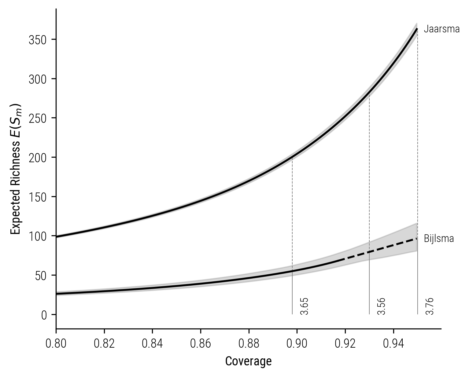
Figure 8: Coverage-based rarefaction-extrapolation curve for Jaarsma and Bijlsma.
The disparity in richness between the collections of Jaarsma and Bijlsma is notably significant. When examining other pairs of collectors, the differences in richness are generally smaller. However, it’s consistently observed that the coverage-based richness estimates are higher compared to those derived from size-based methods. For instance, consider the comparison between the collections of Wever, who focused on gathering stories in the northeastern part of the Netherlands, and Kooijman, whose collection mainly comes from the South-Holland province.
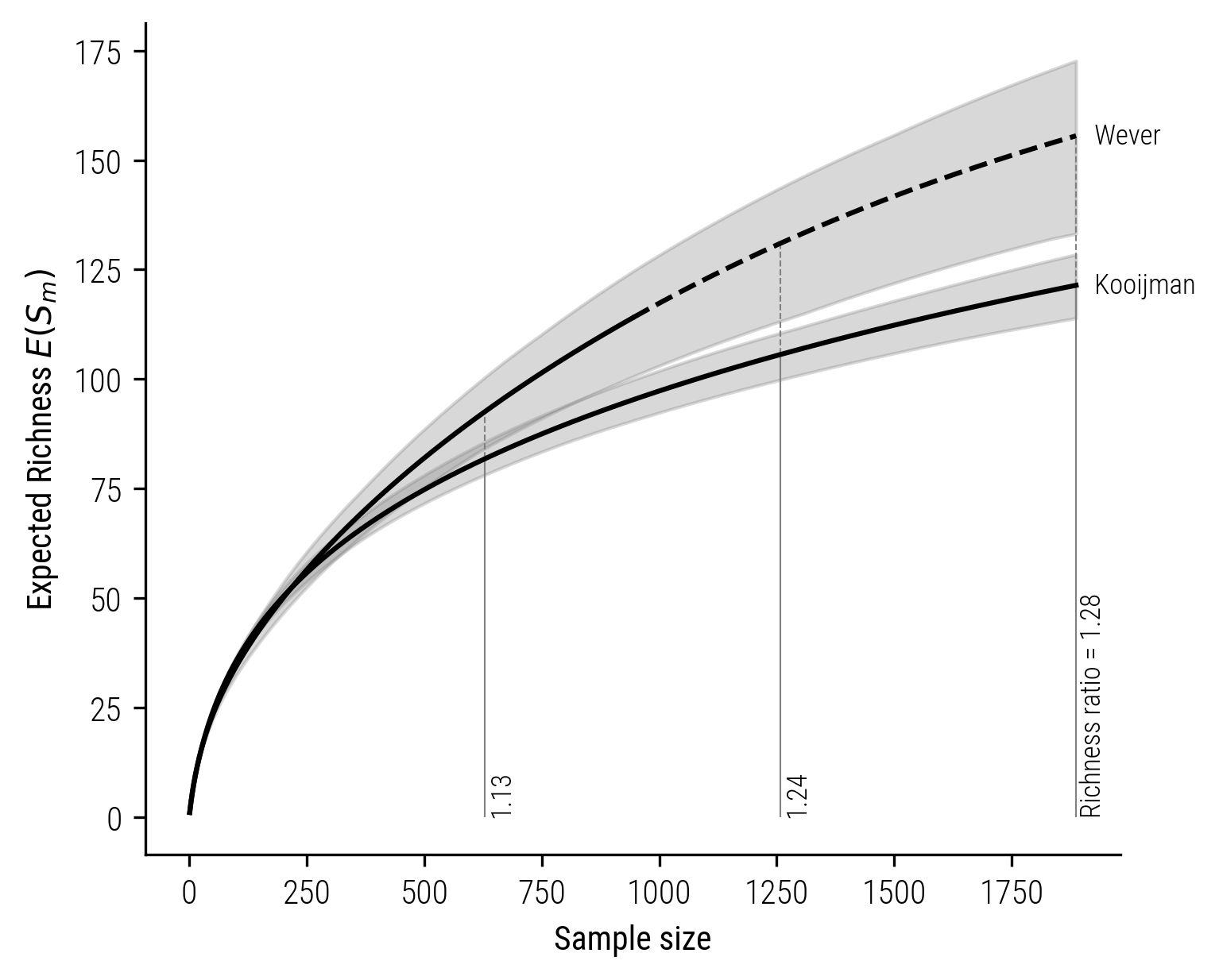
Figure 9: Size-based rarefaction-extrapolation curve for Kooijman and Wever.
The coverage-based rarefaction-extrapolation curves are as follows:
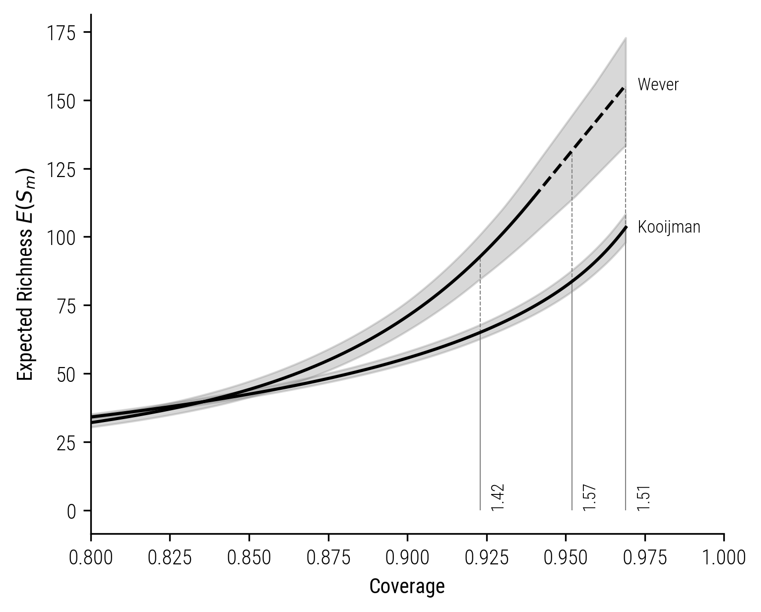
Figure 10: Coverage-based rarefaction-extrapolation curve for Kooijman and Wever.
When comparing these size-based and coverage-based numbers, Chao and Jost (2012) emphasize a key distinction in their approach: while size-based standardization depends on the samplers’ discretion, coverage-based standardization allows for comparisons of equivalent population fractions from each community. This fraction represents a characteristic at the community level, one that can be reliably estimated from the available data.
Outlook
This notebook has delved into the complexities of measuring cultural diversity, with a special focus on a distinctive collection of Dutch folktales. In upcoming posts, I plan to delve deeper into the various factors that influence coverage and diversity within such collections. A key aspect of this exploration will be examining the roles and sampling strategies of the collectors themselves.