Unseen heterogeneity
Unseen Species Models such as Chao1 provide accurate point-estimates of the population size when the rare species in studied sample are homogeneous. That is, in the case of animal species, for example, all species are equally likely to be observed. Of course, this is a simplifying assumption. Some species are simply more difficult to spot than others, and so most samples contain unseen heterogeneity. When such heterogeneity is present in a sample, the Chao1 estimate reduces to a lower bound of the actual population size. What happens when we do have knowledge about (some parts of) the the origin of the heterogeneity? Is there a way to use that information to correct for some of the bias of Chao’s estimator?
In a series of articles, Dankmar Böhning and colleagues show how information about covariates (e.g., certain characteristics of animal species) can help to reduce this bias (Böhning and van der Heijden 2009; Bohning et al. 2013). The crucial insight in these articles is the conceptualisation of Unseen Species Models as maximum likelihood estimators for a truncated Poisson likelihood. That insight allows Bohning et al. (2013) to develop a regression method for population size estimation that incorporates information about covariates and is a generalization of Chao1. Simlarly, Böhning and van der Heijden (2009) use this insight to generalize the Zelterman estimator (Zelterman 1988) to incorporate information about covariates. Below, I will briefly describe both generalizations, after which I will put them to test in a simulation study.
Unseen Species Models in a Likelihood Framework
The Chao1 estimator
As I described in more detail in Demystifying Chao1 with Good-Turing, the Chao1 estimator developed in Chao (1984) takes the form of \(f^2_1 / (2f_2)\), where \(f_1\) indicates how many species occur once, and \(f_2\) how many occur exactly 2 times. The estimator thus only works with \(f_1\) and \(f_2\) (everything that occurs more often, or not at all, is ignored), and that is why we can speak of a truncated distribution. To be more specific: Chao1 assumes that the observed species follow a Poisson distribution, and thus by only considering \(f_1\) and \(f_2\), we are dealing with a truncated Poisson distribution. A Poisson distribution has one parameter \(\lambda\) that represents the expected outcome value, such as the expected number of observations or sightings of an animal species:
\begin{equation} y \sim \text{Poisson}(\lambda) \end{equation}
An exciting insight from Bohning et al. (2013) is that in the case of a truncated Poisson distribution, the parameter \(\lambda\) can be estimated with a binomial likelihood. To understand this, we need to consider that a truncated Poisson with \(y \in {1, 2}\) is in fact a binomial distribution with a binary outcome: something occurs once of something occurs twice. We can thus calculate the probability that something occurs twice and not once, i.e., \(P(y=2)\). That probability is maximised by \(\hat{p} = f_2 / (f_1 + f_2)\). With \(\lambda = 2p/(1 - p)\), we can use \(p\) to obtain an estimate for \(\lambda\).
Bohning et al. (2013) subsequently show that can also estimate \(\hat{p}\) using logistic regression (see also Böhning and van der Heijden 2009). And by doing so, it becomes possible to include information on covariates. These covariates, then, provide information about the probability of an item occuring once or twice in the sample under investigation. In a logistic regression, the outcome probability \(p_i\) is connected to a linear model via a logit link:
\begin{align*} y_i & \sim \text{Binomial}(1, p_i) \\ \text{logit}(p_i) & = \alpha \\ \end{align*}
where \(\alpha\) represents the intercept. This specification allows us to easily add covariates (also called predictors) to the linear model as follows:
\begin{align*} y_i & \sim \text{Binomial}(1, p_i) \\ \text{logit}(p_i) & = \alpha + \beta_x x_i\\ \end{align*}
where \(x_i\) represents the value of a given predictor and \(\beta_x\) the coefficient of predictor \(x\). After estimating \(p_i\) we can estimate the parameter \(\lambda_i\) with:
\begin{equation} \hat{\lambda}_i = 2 \frac{\hat{p}_i}{1 - \hat{p}_i} \end{equation}
What remains is to use the estimate \(\lambda_i\) to calculate the number of unseen items, \(f_0\). Bohning et al. (2013) show that \(f_0\) and the population size \(\hat{N}\) can be estimated with:
\begin{equation} \hat{N} = n + \sum^{f_1 + f_2}_{i = 1} \frac{1}{\hat{\lambda}_i + \hat{\lambda}_i^2 / 2} \end{equation}
For proofs and theorems of this equation, I refer to the note by Bohning et al. (2013). In the remainder of this notebook, I want to concentrate on showing how \(\lambda_i\) and \(p_i\) can be estimated in practice using a Bayesian generalised linear model.
The Zelterman estimator
In Zelterman’s Estimator of Population Size, I briefly introduced the Zelterman estimator, which, combined with the Horvitz-Thompson estimator, can be used as an estimator of the population size, \(\hat{N}\). Böhning and van der Heijden (2009) apply the same framework to develop a version of the Zelterman estimator which can incorporate information about covariates. Recall the the Horvitz-Thompson estimator takes the form of:
\begin{equation} \hat{N} = \frac{n}{1 - e^{-\lambda}} \end{equation}
Thus, we can use the same binomial regression framework to estimate the probability \(p\) that something occur twice and not once, which is uniquely connected to \(\lambda = 2p/(1 - p)\) (see Böhning and van der Heijden 2009 for further details).
Experimenting with Bayesian regression
Simulation Model
In this section, I aim to get a better idea of the effect of heterogeneity in a sample on
the quality of population size estimation. In order to do so systematically, it is useful
to define a function with which we can simulate data. Below, I define a simple function in
Python, generate_population, which lets us generate populations of size \(N\) in which the
number of occurrences of each item \(i\) is sampled from a Poisson distribution:
een Poisson verdeling:
\begin{align*} N_i & \sim \text{Poisson}(\lambda_i) \\ \text{log}(\lambda_i) & = \alpha + \beta x_i \\ \end{align*}
In this equation, \(\alpha\) represents the log-scale intercept (i.e., the mean expected abundance on a log scale), and \(\beta\) the effect (the slope) of predictor \(x\). \(x_i\) takes on a binary value, thus representing two categories (e.g., male en female animals). A translation into Python code is as follows:
import numpy as np
import pandas as pd

def generate_population(N, alpha, beta):
    X = np.zeros(N)
    X[N//2:] = 1
    Lambda = np.exp(alpha + beta*X)
    counts = np.random.poisson(Lambda, size=N)
    return pd.DataFrame({"counts": counts, "X": X})
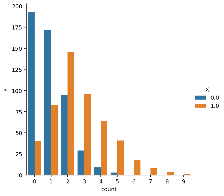
Let’s test the function. Below, I generate a population of 1000 unique items. To first get a feel for how the estimator works with heterogeneity, we’ll set beta to 1:
import seaborn as sns

pop = generate_population(1000, 0, 1)

ax = sns.catplot(
    data=pop.groupby("X")["counts"].value_counts().reset_index(name="f"),
    kind="bar", x="counts", y="f", hue="X")
ax.set(xlabel="count", ylabel="f");
The total number of unseen items as well the number os unseen items per group can be recovered with:
print(f'Total number of missing items is {(pop["counts"] == 0).sum()}')
print(f'Number of missing items with X=1 is {((pop["counts"] == 0) & (pop["X"] == 1)).sum()}')
print(f'Number of missing items with X=0 is {((pop["counts"] == 0) & (pop["X"] == 0)).sum()}')
Total number of missing items is 233
Number of missing items with X=1 is 40
Number of missing items with X=0 is 193
Thus, the chance of unseen items with \(x_i=1\) is much smaller than when \(x_i=0\).
Data preparation
As said, we aim to estimate the parameters of the truncated Poisson distribution by means of logistic regression. To this end, we reduce our generate sample to only contain items that occur once or twice. And subsequently, we add a binary indicator variable \(y\) that equal 1 if the count of item \(i\) is 2, and 0 otherwise. This binary variable, then, will be the outcome variable in the binomial regression model.
data = pop.copy()[pop["counts"].isin((1, 2))]
data["y"] = (data["counts"] == 2).astype(int)
data = data.reset_index(drop=True)
data.sample(5).head()
| counts | X | y | |
|---|---|---|---|
| 275 | 2 | 1 | 1 |
| 163 | 1 | 0 | 0 |
| 360 | 1 | 1 | 0 |
| 65 | 1 | 0 | 0 |
| 226 | 1 | 0 | 0 |
Regression model
We will use the PyMC3 library for doing probabilistic programming in Python to perfom our regression analysis and thus to estimate the parameter \(\hat{p}_i\) and corresponding parameter \(\lambda_i\) through \(\hat{\lambda}_i = 2 \frac{\hat{p}_i}{1 - \hat{p}_i}\). PyMC3 has an intuitive model specification syntax, which allows us to easily code down our model, while maintaining flexibility:
import pymc3 as pm

with pm.Model() as model:
    alpha = pm.Normal('alpha', 0, 5)  # prior on alpha
    beta = pm.Normal('beta', 0, 5)  # prior on beta
    p = pm.Deterministic("p", pm.math.invlogit(alpha + beta*data["X"]))
    f2 = pm.Binomial("f2", 1, p, observed=data["y"])
    trace = pm.sample(1000, tune=2000, return_inferencedata=True)
I assume that most lines of code in this model definition are easy to understand. The deterministic variable \(p\) is there for convenience allowing us to work with estimated values on the probability scale later on. PyMC3 is closely integrated with the ArviZ library, which is the go-to library in Python for exploratory analyses of Bayesian models.
import arviz as az
az.summary(trace, var_names=["alpha", "beta"])
| mean | sd | hdi_3% | hdi_97% | mcse_mean | mcse_sd | ess_bulk | ess_tail | r_hat | |
|---|---|---|---|---|---|---|---|---|---|
| alpha | -0.59 | 0.131 | -0.841 | -0.354 | 0.003 | 0.002 | 1602 | 2034 | 1 |
| beta | 1.15 | 0.196 | 0.758 | 1.491 | 0.005 | 0.004 | 1422 | 1724 | 1 |
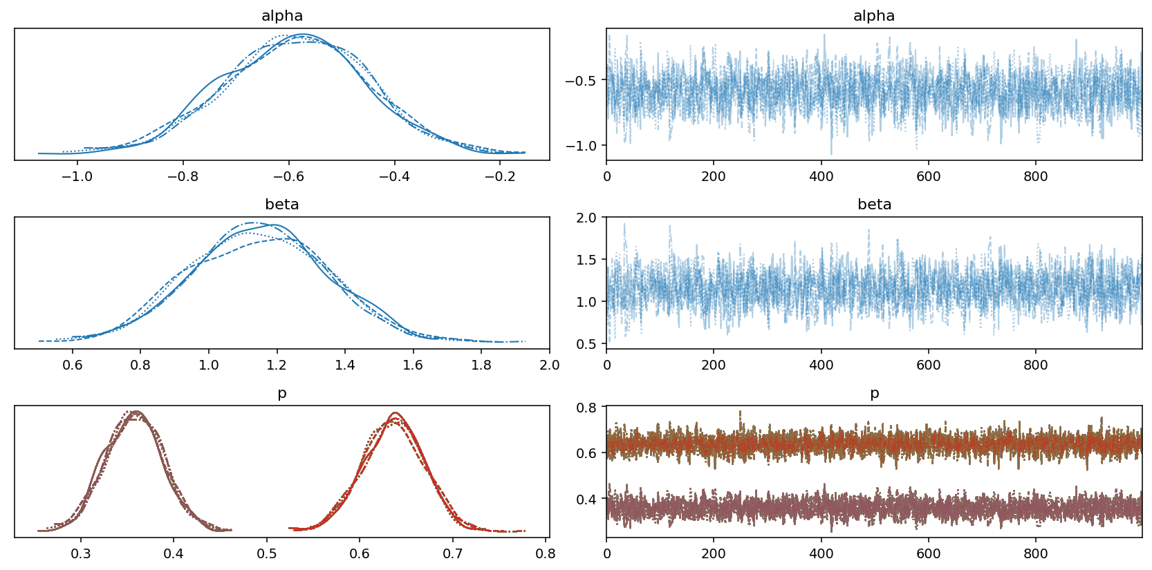
Looking at the table, it appears that the sampling process was succesful, which is also confirmed by the good mixing of the chains in the following trace plot:
az.plot_trace(trace)
plt.tight_layout();
Now that we have an estimate of \(\hat{p}\), we can use that to obtain our estimate of the population size following the equations above. First, we extract 1,000 posterior samples from each chain resulting in 4,000 posterior samples. We then compute the \(\lambda_i\) values for each item \(i\) in the data set. And finally, we compute \(f_0\) and add that to the observed population size to obtain an estimate of the true population size.
post = az.extract_dataset(trace) # stack all chains
n = (pop["counts"] > 0).sum()
p = post["p"].values
l = (2 * p) / (1 - p)
f0 = (1 / (l + (l**2) / 2))
N = n + f0.sum(0)
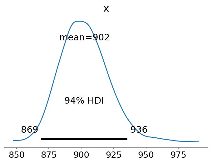
az.plot_posterior(N, point_estimate="mean");
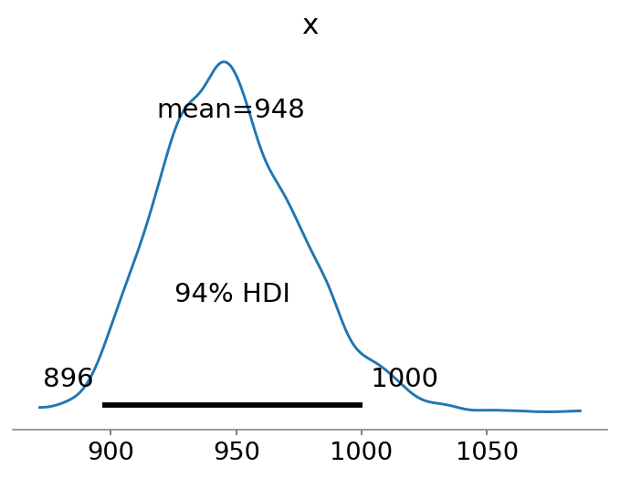
The cool thing about using a Bayesian regression analysis is that our estimate of \(\hat{N}\) becomes a distribution of estimates. We observe that the mean estimate is relatively close to the true value of \(N=1000\).
Note that the estimate is rather similar to the lower-bound of Chao1, which has a slightly more negative bias:
import copia

print(round(copia.chao1(pop["counts"])))
901
An additional benefit of the regression approach is that we can easily obtain posterior population size estimates for different covariates. Below, we plot the estimates for \(x=0\) (left panel) and \(x=1\) (right panel).
fig, axes = plt.subplots(ncols=2, figsize=(8, 4))

labeller = az.labels.MapLabeller(var_name_map={"x": r"$x=0$"})

n0 = ((pop["counts"] > 0) & (pop["X"] == 0)).sum()
l = (2 * p) / (1 - p)
f0_x0 = (1 / (l + (l**2) / 2)) * (data["X"] == 0).astype(int).values[:, None]
S_x0 = n0 + f0_x0.sum(0)

az.plot_posterior(S_x0, ax=axes[0], labeller=labeller);

labeller = az.labels.MapLabeller(var_name_map={"x": r"$x=1$"})
n1 = ((pop["counts"] > 0) & (pop["X"] == 1)).sum()
l = (2 * p) / (1 - p)
f0_x1 = (1 / (l + (l**2) / 2)) * (data["X"] == 1).astype(int).values[:, None]
S_x1 = n1 + f0_x1.sum(0)

az.plot_posterior(S_x1, ax=axes[1], labeller=labeller);
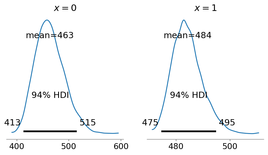
Note that the mean estimates of the two groups add up to the global estimate of the population size. This, however, is not the case when we apply Chao1 to each group individually:
N0 = round(copia.chao1(pop.loc[pop["X"] == 0, "counts"]))
N1 = round(copia.chao1(pop.loc[pop["X"] == 1, "counts"]))

print(f"Estimate for N for X=0 equals {N0}")
print(f"Estimate for N for X=1 equals {N1}")
print(f"The sum of the group estimates equals {N0 + N1}.")
Estimate for N for X=0 equals 461
Estimate for N for X=1 equals 484
The sum of the group estimates equals 945.
Evaluation
A major advantage of the regression approach and certainly regression in a Bayesian framework is that it makes all the usual tools for model evaluation and model comparison available. In this way, it becomes possible to more accurately and systematically investigate whether the assumption of certain covariates leads to a better predictive model, and thus whether the assumption of heterogeneity in the dataset was justified and possibly even necessary to arrive at less biased population size estimates.
ArviZ implements several well-known evelation criteria, such as WAIC and Leave-one-out Cross-validation (LOO). Below, I compare two models using LOO: one with only an intercept (effectively assuming homogeneity), and the previously presented model with an additional coefficient \(\beta\). Before we proceed, let’s fit the intercept-only model:
with pm.Model() as intercept_model:
    alpha = pm.Normal('alpha', 0, 5)  # prior on alpha
    p = pm.Deterministic("p", pm.math.invlogit(alpha))
    f2 = pm.Binomial("f2", 1, p, observed=data["y"])
    intercept_trace = pm.sample(1000, tune=2000, return_inferencedata=True)
The model appears to have converged decently:
import arviz as az
az.summary(intercept_trace, var_names=["alpha"])
| mean | sd | hdi_3% | hdi_97% | mcse_mean | mcse_sd | ess_bulk | ess_tail | r_hat | |
|---|---|---|---|---|---|---|---|---|---|
| alpha | -0.056 | 0.09 | -0.225 | 0.11 | 0.002 | 0.002 | 1612 | 2631 | 1 |
Without coefficients, the regression version of Chao1 reduces to the original Chao1 estimate (Bohning et al. 2013). Thus, unsurprisingly yet reassuringly, the mean estimate of the intercept model is approximately equal to the point-estimate of Chao1:
post = az.extract_dataset(intercept_trace) # stack all chains
n = (pop["counts"] > 0).sum()
nu  = (post["alpha"].values * np.ones(data.shape[0])[:, None])
p = np.exp(nu) / (1 + np.exp(nu))
l = (2 * p) / (1 - p)
f0 = (1 / (l + (l**2) / 2))
N = n + f0.sum(0)

az.plot_posterior(N, point_estimate="mean");
ArviZ provides the neat function az.compare() to compare the out-of-sample predictive
fit of different models. Here, we compute the LOO for both models and display the results
in a DataFrame:
loo_comparison = az.compare(
    {
        "covariate-model": trace,
        "intercept-model": intercept_trace,
    })
loo_comparison
| rank | loo | p_loo | d_loo | weight | se | dse | warning | loo_scale | |
|---|---|---|---|---|---|---|---|---|---|
| covariate-model | 0 | -324.945 | 2.0769 | 0 | 0.967038 | 6.17537 | 0 | False | log |
| intercept-model | 1 | -343.226 | 1.00932 | 18.2808 | 0.0329623 | 0.627712 | 6.1465 | False | log |
The covariate model is ranked first, and received almost all of the weight (which can loosely be interpreted as the probability of a model being true compared to the other model and given the data). Thus, the model comparison confirms what we already knew: the data is heterogeneously generated, and knowlegde about the nature of this heterogeneity should help specifying a better model.
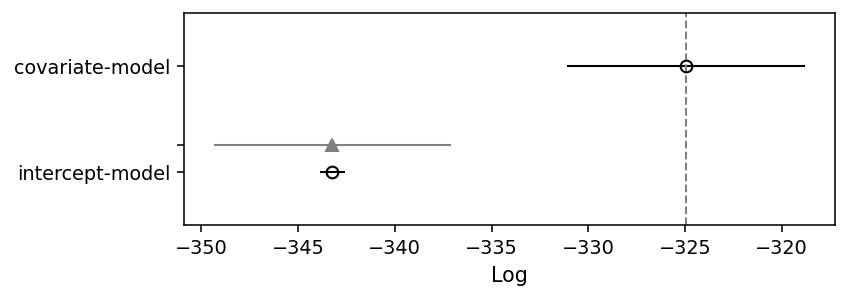
ArviZ also provides a function to create a summary plot much like the ones in McElreath (2018)’s Statistical Rethinking book. The open circles in the plot below represent the LOO values, and the error bars represent the standard deviation of these LOO values. Again, the plot confirms what we already knew, but that’s reassuring if we want to apply the method to real-world case.
az.plot_compare(loo_comparison, insample_dev=False);