Zelterman’s Estimator
In Demystifying Chao1 with Good-Turing, I introduced and explained the Chao1 estimator as an example of a well-known model for estimating the number of unseen species. In this notebook, I study some aspects of another, alternative estimator developed in Zelterman (1988), which has been popular in applications such as drug user studies. This estimator has particular properties that make it more robust or less sensitive to violations of the underlying model. As such, it would be interesting to study how well the estimator performs when applied to cultural data. In what follows, I base my descriptions on the original paper by Zelterman (1988) as well as the more recent application of the method by Böhning and van der Heijden (2009).
All unseen species estimators are based on estimating the probability of an item not being observed, i.e. \(p(y = 0)\). Inversely, the probability that we do observe an item then equals \(1 - p(y = 0)\). It follows that the population size \(N\) is equal to \((1 - p(y = 0)) N + p(y = 0) N\). In other words, the population size is the sum of the fraction of unseen items and the fraction of seen items. This can be rewritten to \(n + p(y=0) N\), since \(n\) represents the observed and thus known population size. Given information about \(n\) and \(p(y=0)\), Horvitz and Thompson (1952) demonstrate that \(N\) can be estimated with:
\begin{equation} \hat{N} = \sum^n_{i = 1} \frac{1}{p(y_i > 0)}. \end{equation}
Here, each item \(i\) is weighted by the inverse of its observation probability. If all items have the same observation probability \(p(y > 0)\), this can be simplified to:
\begin{equation} \hat{N} = \frac{n}{1 - p(y=0)} \end{equation}
To be able to compute this equation, we require knowledge of \(p(y=0)\), and if that’s not available, we need to estimate it. If we assume that the counts \(y\) follow a Poisson distribution, this amounts to estimating \(e^{-\lambda}\), with \(\lambda\) being the Poisson rate parameter. When the counts \(y\) follow a homogeneous Poisson, we can estimate \(\lambda\) with maximum likelihood (Böhning and van der Heijden 2009). However, this homogeneous assumption is often violated, as not all values of \(y\) adhere to the Poisson distribution.
This is where Zelterman (1988) comes in. Zelterman argues that while the Poisson assumption might not be valid for the complete range of \(y\), it may apply to smaller ranges, such as from \(r\) to \(r + 1\). If we represent the number of items occurring \(r\) times as \(f_r\), Zelterman proposes to use \(f_r\) and \(f_{r + 1}\) to estimate \(\lambda_r\). Thus, to estimate \(\lambda_{r = 1}\), we can use:
\begin{equation} \hat{\lambda}_1 = \frac{(r+1)f_{r + 1}}{f_r} = \frac{2f_2}{f_1}. \end{equation}
Interestingly, \(\hat{\lambda}_r\) is computed using the exact same formula as Turing and Good proposed to obtain their unnormalized, adjusted counts \(r^*\) (see Good 1953 and Demystifying Chao1 with Good-Turing). Zelterman’s estimator of \(\lambda\) is said to be robust as it only takes into account items that occur once or twice, and as such deviations from the Poisson in higher order counts do not impact the estimation. Put differently, the distribution only needs to look like a Poisson for \(f_1\) and \(f_2\). If we plug Zelterman’s estimate of \(\lambda\) into the estimator by (Horvitz and Thompson 1952), we obtain an estimate of the population size \(\hat{N}\) with \(\frac{n}{1 - e^{-\hat{\lambda}}}\) (see Böhning and van der Heijden 2009 for further details).
Testing the Zelterman estimator
To get a feeling of how the Zelterman estimator behaves, let’s apply it to some simulated data. Below, I define a function in Python which generates a population that follows a Poisson distribution:
import numpy as np

def generate_population(V, alpha):
    counts = np.random.poisson(np.exp(alpha), size=V)
    return {"counts": counts, "V": V, "N": counts.sum()}

pop = generate_population(100, 0)
Using this function we can generate populations, such as the following:
import pandas as pd

ax = pd.Series(pop["counts"]).value_counts().sort_index().plot(kind="bar")
ax.set(xlabel="$r$", ylabel="$f_r$");
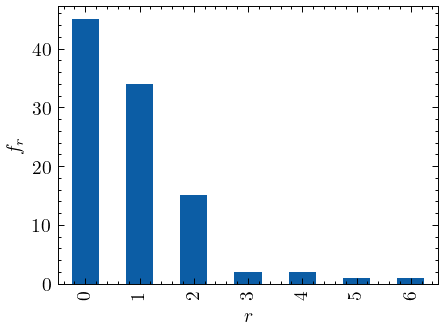
Total number of observed items n = 89
Total number of unique items V = 100
Total number of missing items is 45
We will use the Zelterman estimator to obtain estimates for \(\hat{N}\) and \(\hat{V}\). The estimator is easy to implement, as demonstrated by the following lines of code:
def horvitz_thompson_estimator(n, l):
    return n / (1 - np.exp(-l))

def zelterman_estimator(f1, f2):
    return (2 * f2) / f1

def estimate_population_size(x):
    x = x[x > 0]
    f1 = (x == 1).sum()
    f2 = (x == 2).sum()
    l = zelterman_estimator(f1, f2)
    return {
        "N": horvitz_thompson_estimator(x.sum(), l),
        "V": horvitz_thompson_estimator(x.shape[0], l)
    }
Applying the estimator to our simulated population, we obtain the following estimates of \(V\) and \(N\):
estimate_population_size(pop["counts"])
| N | : | 151.82741330117702 | V | : | 93.8259295681431 |
Note that these estimates are very similar to the ones obtained by applying the Chao1 estimator:
| N | : | 127.1003745318352 | V | : | 93.1003745318352 |
How many words did Shakespeare know?
In the 1970s. pioneers Efron and Thisted applied Unseen Species Models to cultural data. In Efron and Thisted (1976), they attempt to estimate how many unique words Shakespeare knew but did not use. How large, so to speak, was his passive vocabulary, and how large was his total vocabulary? Efron and Thisted (1976) estimate these numbers in part based on the Good-Turing estimator (see Demystifying Chao1 with Good-Turing). They calculate that Shakespeare must have known at least approximately 35,000 additional words on top of the 31,543 he used in his works.
Below, I will apply the Zelterman estimator to make an alternative estimate of Shakespeare’s vocabulary. For this purpose, I will use the word counts as mentioned in Efron and Thisted (1976):
| \(f_1\) | \(f_2\) | \(V\) | \(N\) |
|---|---|---|---|
| 14,376 | 4,343 | 31,534 | 884,647 |
Based on these counts, we can easily plug the numbers into the Zelterman formula. We first calculate \(\lambda_{r = 1}\) with \(\lambda_{r=1} = (2 \times 4343) / 14376 = 0.6042\). Subsequently, we apply the Horvitz-Thompson estimator to arrive at our estimate of the vocabulary: \(\hat{V} = 31534 / (1 - \text{exp}(-0.6042)) = 69536\) unique words. With this, the Zelterman estimator estimates Shakespeare’s vocabulary as being slightly larger, but in the same ballpark as the one by Efron and Thisted (1976).