Unseen Species Models such as Chao1 assume that the sample being studied was created with replacement. This means that calculations are based on the assumption that certain individuals can or have been repeatedly observed. It also implies that the observation of one individual does not influence the observation of the next individual. That is to say: observations are independent. Take, for example, an ecologist who wants to use Chao1 to estimate the number of unique animal species that live in a given environment. Assuming for the moment that the presence of the researcher in that environment does not introduce any observation biases, we can think of the observation process as a sample with replacement: upon registration, animals are re-placed into the environment, and thus there is chance that ecologist is observing the same animal twice.
However, it also happens that animals, in particular insects, are killed upon capture. In that case, the assumption of sampling with replacement no longer holds. Individuals are no longer independently sampled, meaning that the capture of one invidividual (positively or negatively) impacts the capture probability of another individual. When applied to the cultural domain, and especially when working with cultural collections, one could argue that the assumption of sampling with replacement is often quite problematic. Cultural collections are, by definition, finite samples created without replacement. The same applies to the example of estimating the vocabulary size of a text based on a snippet of text, as I explained in an earlier post (see Demystifying Chao1 with Good-Turing). Here, too the assumption of replacement is clearly violated.
This isssue of recognizing which sampling strategy underlies our data potentially has major implications for the quality of the estimates made by unseen species models. In Kestemont et al. (2022), for example, we assume that the samples we have of medieval narratives are the result of a sampling process with replacement. Clearly, this is not realistic. The question, then, is to what extent this assumption impacts the estimates. In this notebook, I try to get a better idea of the impact of sampling strategies on the quality and bias of estimates computed with Chao1. I will show that when samples are created without replacement and the sample fraction is relatively large, Chao1 no longer forms a lower-bound and thus greatly overestimates the true richness. However, when the sampling fraction is small, Chao1 remains a lower-bound and the difference between samples with and without replacement is negligible. To compensate for estimation biases introduced by sampling without replacement, I investigate the Unseen Species Model proposed by Chao and Lin (2012), which was specifically desgined to work with samples created without replacement.
Chao & Lin (2012)
Chao and Lin (2012) describe an Unseen Species Model based on Chao1 with which we can compute a lower-bound estimate of the number of unseen items (e.g., species, cultural artifacts) in samples created without replacement. The formula is closely related to the original Chao1 estimator (see Demystifying Chao1 with Good-Turing for further details):
\begin{equation} \hat{V} = V_{\textrm{obs}} + \frac{f^2_1}{\frac{n}{n - 1} 2f_2 + \frac{q}{1 - q} f_1} \end{equation}
Here, \(V_{\textrm{obs}}\) represents the observed number of unique items. \(f_1\) is the number of items that occurs exactly once in the sample, and \(f_2\) is the number of items that occurs twice in the sample. The size of the sample is denoted with \(n\), and \(q\) represents the sample fraction. Thus, \(q\) assumes we have knowledge about the true population size \(N\). We can easily implement the model in Python:
import numpy as np

def chao_wor(x, q):
    x = x[x > 0]
    n = x.sum() # sample size
    t = len(x)  # number of unique items
    f1 = (x == 1).sum() # number of singletons
    f2 = (x == 2).sum() # number of doubletons
    return t + (f1**2) / ((n / (n - 1)) * 2*f2 + (q / (1 - q)) * f1)
For reference, Chao1 can be implemented using similar lines of code (see the Python package copia or the R package iNEXT for more robust implementations as well as other estimators):
def chao1(x):
    x = x[x > 0]
    n = x.sum()
    t = len(x)
    f1 = (x == 1).sum()
    f2 = (x == 2).sum()
    if f2 > 0:
        return t + (n-1)/n * (f1**2 / (2*f2))
    return t + (n-1)/n * f1*(f1-1) / 2*(f2+1)
Testing the replacement assumption
In what follows, I will use these two models to test the impact of the assumptions underlying the sampling process on the quality of the estimations. Thus, what happens if we apply Chao1 to data that was generated without replacement, while Chao1 asssumes it to be generated with replacement. Although Chao and Lin (2012) also discuss incidence data as well as shared richness estimation, I will primarily focus on the case of abundance data (i.e., counts of (species) types).
By means of illustration, I will apply the models to a case of textual data. Here the goal is the estimate the vocabulary size of some text based on a snippet of that text. Such a snippet can be seen a a contiguous sample created without replacement. This is an interesting application as it allows us to work with real-world data, without having to compromise on having knowledge about the true population and vocabulary size. The text we will be working with is Shakespeare’s Hamlet, which can be downloaded from the Folger Digital Text collection with the following lines of Python code (for more information about parsing this corpus with Python, please see Karsdorp, Kestemont, and Riddell 2021):
import requests
import lxml.etree as etree
import collections

root = "https://shakespeare.folger.edu/downloads/teisimple/"
hamlet = "hamlet_TEIsimple_FolgerShakespeare.xml"
response = requests.get(root + hamlet)
hamlet = etree.fromstring(response.content)

NSMAP = {'tei': 'http://www.tei-c.org/ns/1.0'}
words = [w.text for w in hamlet.iterfind(".//tei:w", namespaces=NSMAP) if w.text is not None]
We transform the text, represented as a list of words, into a NumPy array, and subsequently calculate the length of the text \(N\) as well as the number of unique words \(V\):
counts = np.array(list(collections.Counter(words).values()))
N, V = counts.sum(), counts.shape[0]
print(f"The text consists of N={N} words and V={V} unique words.")
The text consists of N=31928 words and V=5288 unique words.
Chao1 and the replacement assumption
To set a baseline, I will first illustrate how Chao1 performs when estimating the vocabulary size \(V\) for samples of the text generated with replacement. Here we create samples with \(q\) in the range [0.001 0.999], and plot the estimates for different values of \(q\):
import matplotlib.pyplot as plt

def ci_plot(x, y, n=20, percentile_min=1, percentile_max=99,
            color='C0', label=None, ax=None):
    if ax is None:
        fig, ax = plt.subplots()

    perc1 = np.percentile(
        y, np.linspace(percentile_min, 50, num=n, endpoint=False), axis=0)
    perc2 = np.percentile(
        y, np.linspace(50, percentile_max, num=n+1)[1:], axis=0)

    alpha = 1/n
    for p1, p2 in zip(perc1, perc2):
        ax.fill_between(x, p1, p2, alpha=alpha, color=color, edgecolor=None)
        ax.plot(x, np.mean(y, axis=0), color=color, label=label)
    return ax

n_steps, n_experiments = 50, 100
fractions = np.linspace(0.001, 0.999, n_steps)
est_wr = np.zeros((n_experiments, n_steps))
for j, q in enumerate(fractions):
    for i in range(n_experiments):
        _, sample = np.unique(
            np.random.choice(V, size=int(q * N), p=counts/counts.sum()),
            return_counts=True)
        est_wr[i, j] = chao1(sample)

fig, ax = plt.subplots()
ci_plot(fractions, est_wr, n=3, color="C0", ax=ax)
ax.set(ylabel="$\hat{V}$", xlabel="$q$")
ax.axhline(V, color="grey", ls="--");
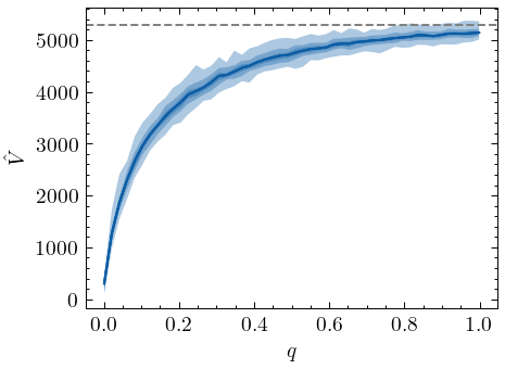
The plot here cleary shows that the Chao1 estimator converges to the true vocabulary size \(V\) as the sample fraction \(q\) increases. Also note that the estimator consistently produces a lower-bound estimate, and that the extent of the negative bias is non-linear. All in all, the estimator seems to perform as solid a lower-bound estimate of the vocabulary size.
When working with texts, however, it is more common to deal with samples created without replacement. Suppose we find a snippet of a text. Such a snippet represents a contiguous sample of the original text, one that was created without replacing words. Let’s investigate what happens if we create a sample without replacement, and use Chao1 to estimate the true value \(V\) based on such a sample:
est_wor = np.zeros((n_experiments, n_steps))
flat_pop = np.repeat(np.arange(V), counts)
for j, q in enumerate(fractions):
    for i in range(n_experiments):
        _, sample = np.unique(np.random.choice(
            flat_pop, replace=False, size=int(q * N)), return_counts=True)
        est_wor[i, j] = chao1(sample)

fig, ax = plt.subplots()
ci_plot(fractions, est_wor, n=3, color="C0", ax=ax)
ax.set(ylabel="$\hat{V}$", xlabel="$q$")
ax.axvline(fractions[np.where(est_wor.mean(0) > V)[0]][0], color="grey", ls="--")
ax.axhline(V, color="grey", ls="--");
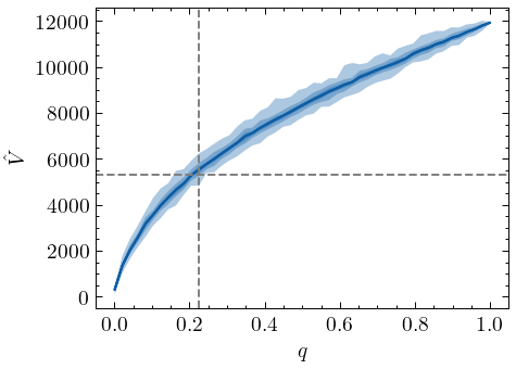
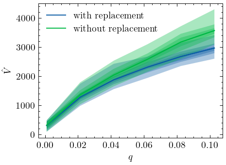
When samples are generated without replacement, Chao1 clearly no longer provides a lower-bound estimate of the vocabulary size for sample fractions \(q \gtrapprox 0.2\). In fact, as the plot illustrates, this positive bias can be quite dramatic for larger fraction sizes. It is important to note, however, that Chao1 still provides a lower-bound of the richness for small sample sizes, and that for these sizes estimates based on sampling with and sampling without replacement do not diverge too much (Kestemont et al. (2022), for example, computed their estimations based on a sample fraction of \(q \approx 0.09\). While their sample may not be created with replacement, this fraction is small enough to employ the Chao1 estimator.):
fig, ax = plt.subplots()

labels = "with replacement", "without replacement"
estimations = est_wr, est_wor

for i, (label, est) in enumerate(zip(labels, estimations)):
    ci_plot(fractions[:6], est[:, :6], n=3, color=f"C{i}", ax=ax, label=label)

ax.set(ylabel="$\hat{V}$", xlabel="$q$")

handles, labels = plt.gca().get_legend_handles_labels()
by_label = dict(zip(labels, handles))
ax.legend(by_label.values(), by_label.keys());
Chao without the replacement assumption
For larger sample fractions, however, Chao1 can greatly overestimate the true diversity in a sample. Precisely to overcome this problem, Chao and Lin (2012) developed their lower-bound estimator for samples without replacement. Below, I will demonstrate how this estimator can be used to deal with samples for which we cannot and should not assume that they were created with replacement. Recall that the estimator of Chao and Lin (2012) assumes that \(N\) is known (or that \(q\) is known, depending on the perspective). If we apply this estimator to our samples created without replacement, we obtain the following graph:
fractions = np.linspace(0.01, 0.999, n_steps)
estimations = np.zeros((n_experiments, n_steps))
flat_pop = np.repeat(np.arange(V), counts)
for j, q in enumerate(fractions):
    for i in range(n_experiments):
        _, sample = np.unique(np.random.choice(
            flat_pop, replace=False, size=int(q * N)), return_counts=True)
        estimations[i, j] = chao_wor(sample, q)

fig, ax = plt.subplots()
ci_plot(fractions, estimations, n=3, color="C0", ax=ax)
ax.set(ylabel="$\hat{V}$", xlabel="$q$")
ax.axhline(V, color="grey", ls="--");
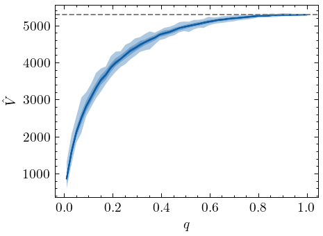
As clearly shown by the graph, if we know \(q\), the modified estimator behaves like Chao1 for samples with replacement and acts as a proper lower-bound of the vocabulary size. But of course, we only rarely know about \(q\) or \(N\). More often, we have no knowledge whatsoever about the true population size. When such information is absent, Chao and Lin (2012) suggest to estimate the vocabulary size using different hypothetical values of \(q\). Below, we generate samples with different values of \(q\), and for each of those, we estimate the vocabulary size using several hypothetical \(q\) values, \(\hat{q}\):
n_steps, n_experiments = 20, 100
fractions = np.linspace(0.01, 0.999, n_steps)
q_hypotheses = np.linspace(0.01, 0.999, 20)
estimations = np.zeros((n_steps, 20))
flat_pop = np.repeat(np.arange(V), counts)
for k, h in enumerate(q_hypotheses):
    for j, q in enumerate(fractions):
        _ests = []
        for i in range(n_experiments):
            _, sample = np.unique(
                np.random.choice(flat_pop, replace=False, size=int(q * N)),
                return_counts=True)
            _ests.append(chao_wor(sample, h))
        estimations[j, k] = np.mean(_ests)
We plot the results as a contour plot:
X, Y = np.meshgrid(fractions, q_hypotheses)
Z = V - estimations

fig, ax = plt.subplots()
ax.contourf(X, Y, Z)
CS = ax.contour(X, Y, Z, colors="w")
ax.clabel(CS, inline=True, fontsize=10)
ax.set(
    xlabel="true fraction",
    ylabel="hypothetical fraction",
    title="Estimation error")
ax.grid()
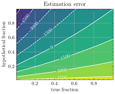
The graph provides important information about the conditions under which the estimator is still a lower-bound. First, we see that if the true fraction \(q\) is small and the hypothetical fraction \(\hat{q}\) is large, the estimates have a (relatively strong) negative bias. Conversely, when the hypothetical fraction is small but the true fraction is larger, the estimator often greatly overestimates the true vocabulary size. Note that positive bias was to be expected with \(\hat{q}\) approaching 0, because then, the estimator approaches the Chao1 estimator, and, Chao1 displays the same positive bias when the sample was generated without replacement. More generally, the plot seems to suggest that if \(\hat{q} \lt q\), the estimator overestimates the true richness, and thus the estimates can no longer be considered lower-bound estimates.