This notebook is the second in a series of notebooks based on a talk I gave at the CUDAN 2023 conference in Tallinn, Estonia (https://cudan.tlu.ee/conference/) together with Melvin Wevers and Mike Kestemont, titled Steady Formulas, Shifting Spells: Estimating Folktale Diversity.
Collector’s curves
In a previous discussion, I delved into how we can use ecological concepts to understand cultural diversity, focusing on what we call ‘cultural richness.’ This term refers to the variety of unique items found in different collections. I illustrated the use of a method developed by Chao and Jost (2012) to compare this richness across collections in a way that doesn’t depend on how much effort the collectors put into gathering their items. This method is based on estimates of the “coverage” of a collection (Good 1953).
One key idea is that the richness of a collection is closely linked to how many items you’ve collected. Generally, the more items you gather, the more unique ones you’re likely to find. This relationship is illustrated using what we call “collector’s curves”, sometimes also known as “species accumulation curves”. These curves show the number of new, unique categories (like species in ecology or folktale types in folklore) we discover as we keep adding more items to our collection.
We can compare these to another type of curve called a “rarefaction curve”. Unlike the collector’s curve, which shows what we actually observe, the rarefaction curve is more about what we might expect to find theoretically as we keep adding more items. Take a look at the graph below. In this fictional example, you can see how the rarefaction curve initially rises quickly. This fast rise happens because we’re finding the most common species. But, as time goes on, the curve levels out because discovering new, rare species becomes harder.
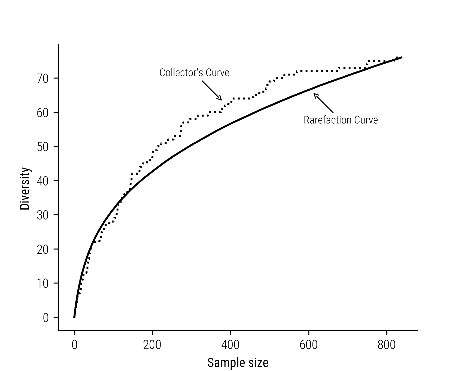
Figure 1: Fictional collector’s curve and its corresponding rarefaction curve.
To create a rarefaction curve, ecologists (and we can use this in cultural studies too) pick random subsets from their total collection and note how many unique species they find in each subset. This process is repeated, gradually increasing the size of the subset, and the average number of species found in each size group is plotted. Essentially, rarefaction curves show us what we might expect to find in a smaller, randomly chosen part of a larger collection.
The main aim of my exploration here is to deepen our understanding of the relationship between what we actually collect (shown in the collector’s curves) and what we might expect to collect if our process were completely random (shown in the rarefaction curves). This is crucial because we know that collectors, whether in cultural or biological contexts, often have certain biases. By studying how actual collections differ from these theoretical curves, I hope to learn something about the nature of these biases.
Exploration versus Exploitation
Rarefaction curves thus serve as a benchmark, showing us the expected diversity in a collection if items were gathered randomly and without any specific focus or bias. It’s a theoretical model that represents an idealized, unbiased collection process. When the actual collector’s curve – the curve showing the number of unique items actually found – deviates from this model, it indicates that the collection process is influenced by certain tendencies or preferences:
-
If the actual curve rises above the rarefaction curve, it suggests that the collection is more diverse than what random sampling would predict. This could mean that the collector is particularly effective at uncovering a wide variety of items, possibly going out of their way to find rare or unique items. It’s a pattern suggesting a proactive approach in seeking diversity, one we might call an “exploration bias”.
-
On the other hand, if the collector’s curve falls below the rarefaction curve, this indicates a narrower scope of collection than what would be expected at random. In this case, the collector might be focusing more on gathering more items or variants of a particular type or category, possibly due to a preference for certain kinds of items or a more limited scope of collection. The bias here could be seen as a form of “exploitation bias”.
The idea is that these deviations are more than just statistical anomalies; they are clues to the collector’s strategy, preferences, and even potential biases. Whether due to personal interest, accessibility, or other factors, these patterns can significantly shape the composition of the collection.
Simulating Collectors
To put this theory into practice and explore how these biases play out in real
collection scenarios, I developed a simple simulation model that allows us to
experiment with different biases in a controlled environment. The sample_items
function below implements a simulation model for a collection process influenced
by a tendency or bias toward novelty or familiarity, or exploration versus
eploitation.
import random

def sample_items(item_universe, sample_size=100, bias=0):
    collection, collection_set = [], set()

    while len(collection) < sample_size:
        sampled_item = random.choice(item_universe)

        is_item_new = sampled_item not in collection_set
        keep_probability = 0.5 + (bias / 2) * (1 if is_item_new else -1)

        if random.random() < keep_probability:
            collection.append(sampled_item)
            collection_set.add(sampled_item)

    return collection
The general idea behind the function is to mimic the collection process by deciding whether to include each potential new item based on a probability that is adjusted by a “bias” parameter \(\beta\). This parameter tilts the balance of the decision-making process:
- A positive value of \(\beta\) leads to a preference for adding new, uncollected items, simulating an explorative behavior.
- A negative \(\beta\) favors the selection of items that have already been collected, simulating a conservative or risk-averse behavior.
- With no bias, the selection is neutral, giving equal opportunity to new and already collected items.
Analyzing the Model
Using the sample_items function, the goal is to observe how varying degrees of
bias influence the diversity of items collected over time, providing us with a
more precise insight into the decision-making patterns in collection processes.
The simulation setup is as follows:
- Bias Range: I explored a range of bias strengths, from \(\beta=-0.9\) (indicating strong exploitation or familiarity bias) to \(\beta=0.9\) (representing strong exploration or novelty bias). This range also included a neutral point (\(\beta=0.0\)), where there was no preference for either new or familiar items.
- Sample Size: Each simulation involves collecting 4,000 items. This sample size was chosen to ensure that each unique item in the universe is likely to be sampled at least once. This consistency is crucial, as it ensures that the rarefaction curves for all simulations is identical, and thus serves as a reliable baseline for comparison.
- Iterations: I repeat each simulation 100 times for each bias setting. This repetition is necessary to average out anomalies and highlight the consistent trends attributable to the biases. We then compute the mean collector’s curves for each bias setting.
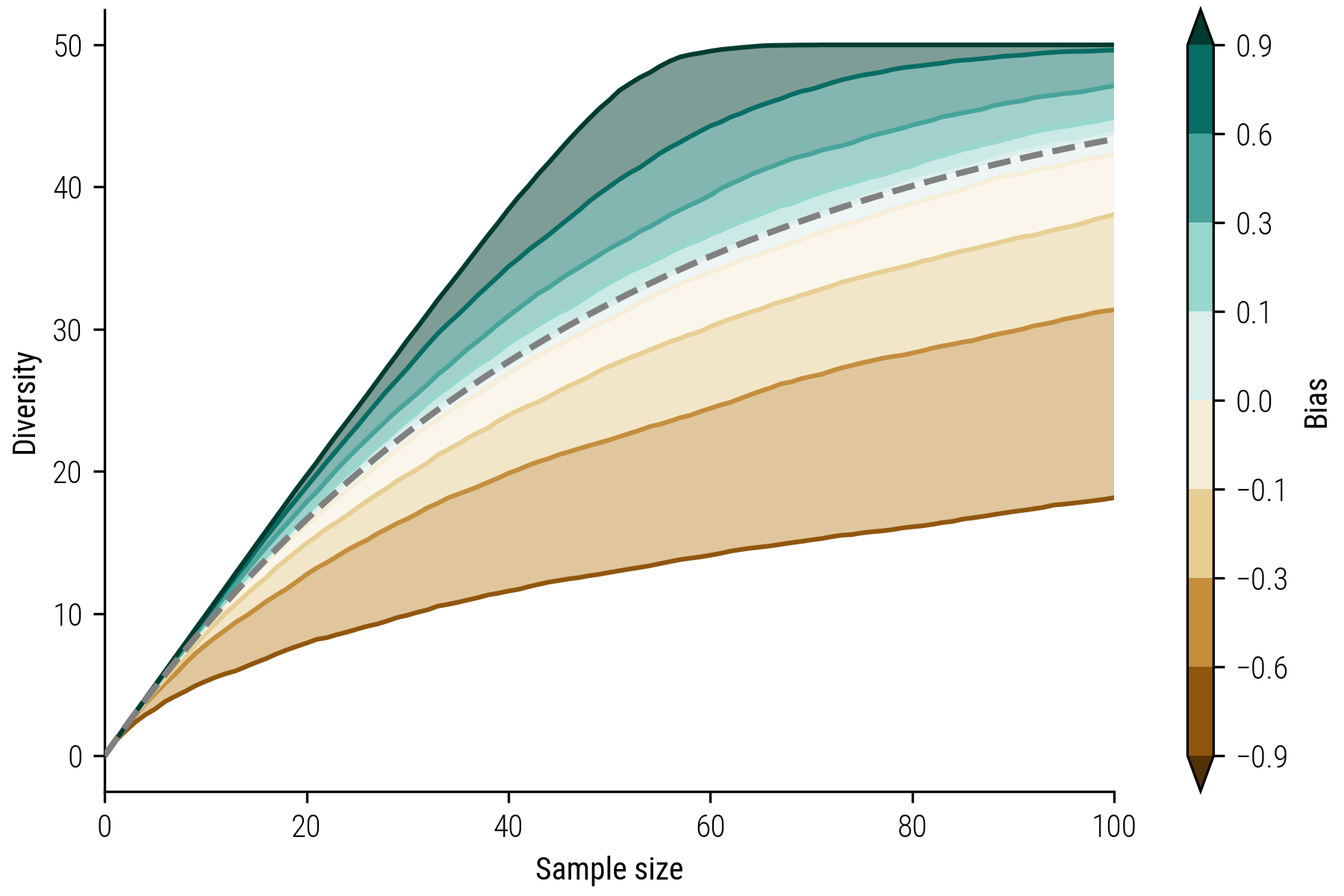
Figure 2: Collector’s curves for different bias values. Positive values indicate a exploration bias, while negative value indicate a exploitation bias. The dashed line displays the rarefaction curve which is the same for all models.
This simulation approach allows us to visualize and quantify the effects of varying biases on collection diversity. The figure above highlights how preferences for novelty (positive bias) or familiarity (negative) can shape the composition of a collection. The dashed line represents the rarefaction curve, which is the same for all collector’s curves. Note that the rarefaction curve is also identical to the situation where a collector has no bias (i.e. \(\beta=0\)).
Biases of Folktale Collectors
In my earlier notebook Coverage-based Comparisons of Cultural Diversity, I touched upon a folklore project undertaken by the Meertens Institute during the 60s and 70s. This ambitious initiative aimed to map Dutch folklore comprehensively, resulting in an atlas of folktales. A team of folktale collectors, appointed by the institute, traversed various regions near their residences to gather these tales. Their mission was to document the stories across the entire Netherlands. This groundbreaking effort in folkloristics amassed a remarkable collection of over 32,000 stories. In this section, I aim to explore the biases in their collection efforts based on their collection’s curves and the relationship with the accompanying rarefaction curves.
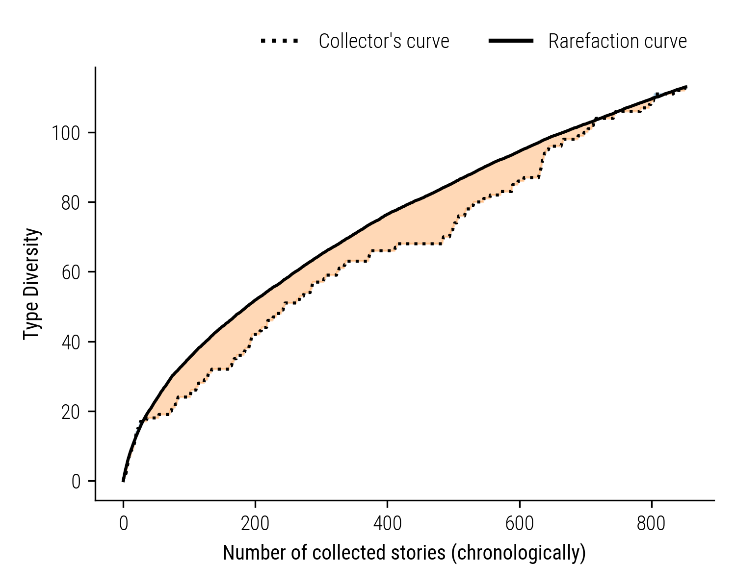
Figure 3: Collector Wever’s Bias Illustrated: The dotted line represents Wever’s actual diversity of collected stories, while the solid line is the theoretical rarefaction curve. The orange area shows segments of conservative collecting, with a preference for familiar story types.
Examining individual collectors, we turn our attention to Wever, who amassed nearly a thousand tales, primarily from the north-eastern region of the Netherlands. The graph above illustrates Wever’s collection trajectory (shown as the dotted line) and juxtaposes it with the expected diversity trend, known as the rarefaction curve (the solid line). The shaded orange area highlights the segments where Wever’s actual diversity of new story types fell short of the number anticipated by a neutral collection model. This suggests that Wever exhibited a tendency towards collecting known story types rather than venturing into new narrative territories.
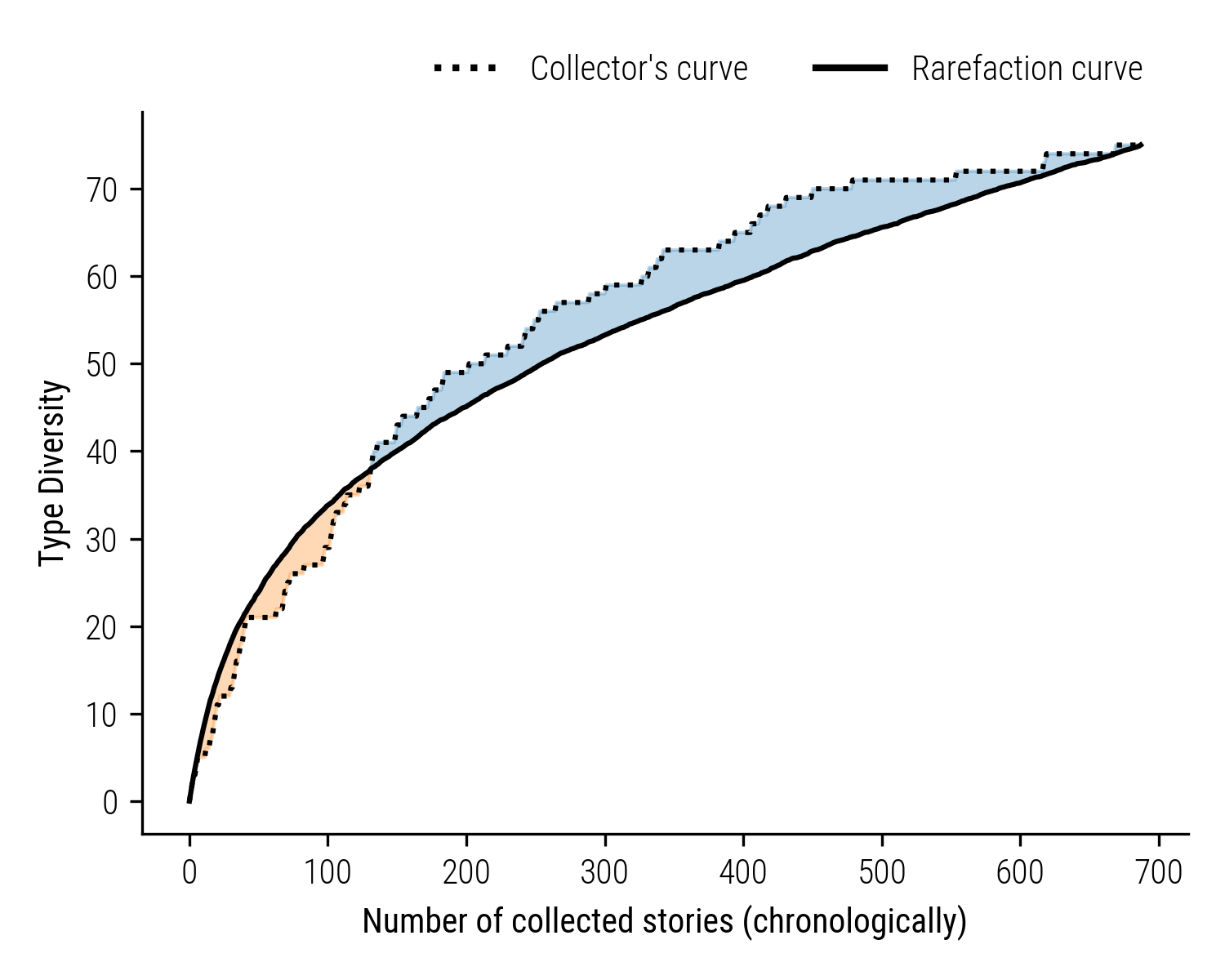
Figure 4: Keuning’s Active Exploration: The dotted line shows the actual diversity of stories collected by Keuning, while the solid line indicates the expected rarefaction curve. The blue shaded area denotes Keuning’s tendency to seek out and collect new story types beyond the neutral model’s prediction.
Keuning’s collection, featuring a comparable number of stories gathered from the northern region of Frysia, presents a contrasting pattern. The graph depicts Keuning’s collector’s curve, which surpasses the theoretical rarefaction curve, suggesting a tendency towards discovering more new story types than one would expect from a neutral, unbiased approach. The phase of active exploration is marked in blue, underscoring Keuning’s inclination towards variety in story collection.
The plot below provides the collectors’ curves and corresponding rarefaction for a number of other collectors.
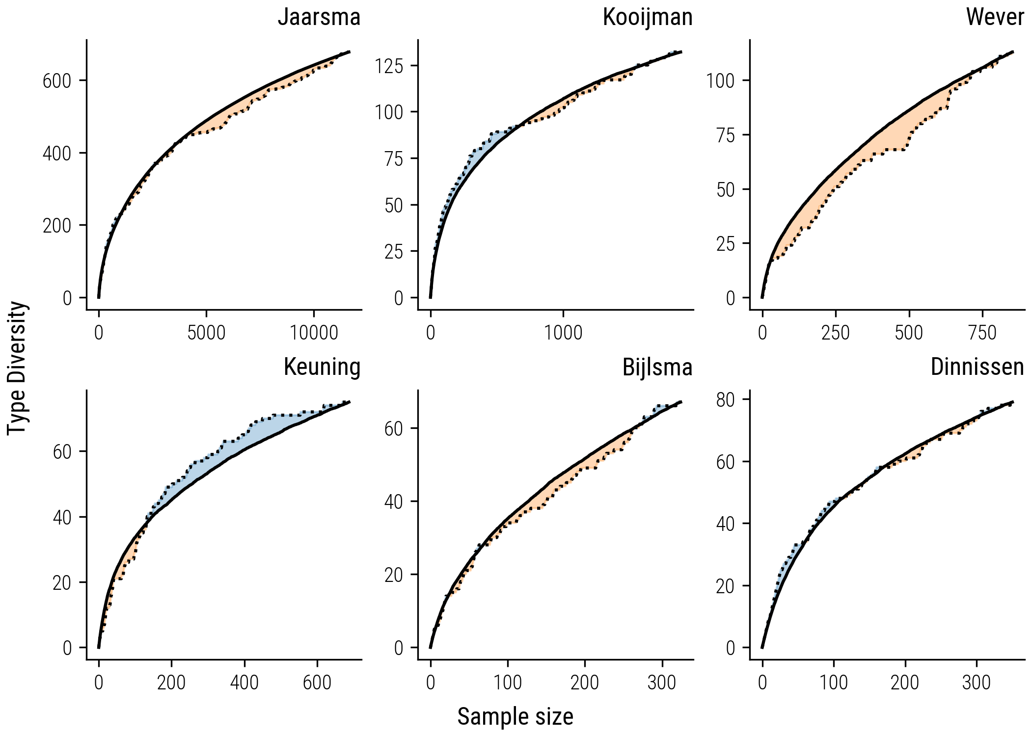
Figure 5: Collectors’ curves and accompaying rarefaction curves.
More than just random fluctuations?
To evaluate whether the observed deviations in the collectors’ curves from the expected rarefaction curve are due to chance or represent a pronounced bias, I use a bootstrapping approach. First, for each collector, we establish an empirical collector’s curve based on the actual data gathered. In parallel, we generate a rarefaction curve reflecting a hypothetical unbiased collection process, where material is collected without any predisposition towards novelty or familiarity.
Subsequently, we initiate the bootstrapping process, creating 1,000 random collector’s curves. This can be accomplished by reshuffling the empirical data 1,000 times, which allows us to simulate the variation one might expect from random chance. For each of these simulated curves, we calculate the difference in the area under the curve (AUC) when compared to the rarefaction curve.
The same difference in AUC is then computed between the empirical collector’s curve and the rarefaction curve. We visualize the distribution of the AUC differences from the bootstrapped curves in a histogram. The histogram below is based on the collection of Wever, we saw before. Here, the overlaid vertical line marks the AUC difference of the empirical collector’s curve.
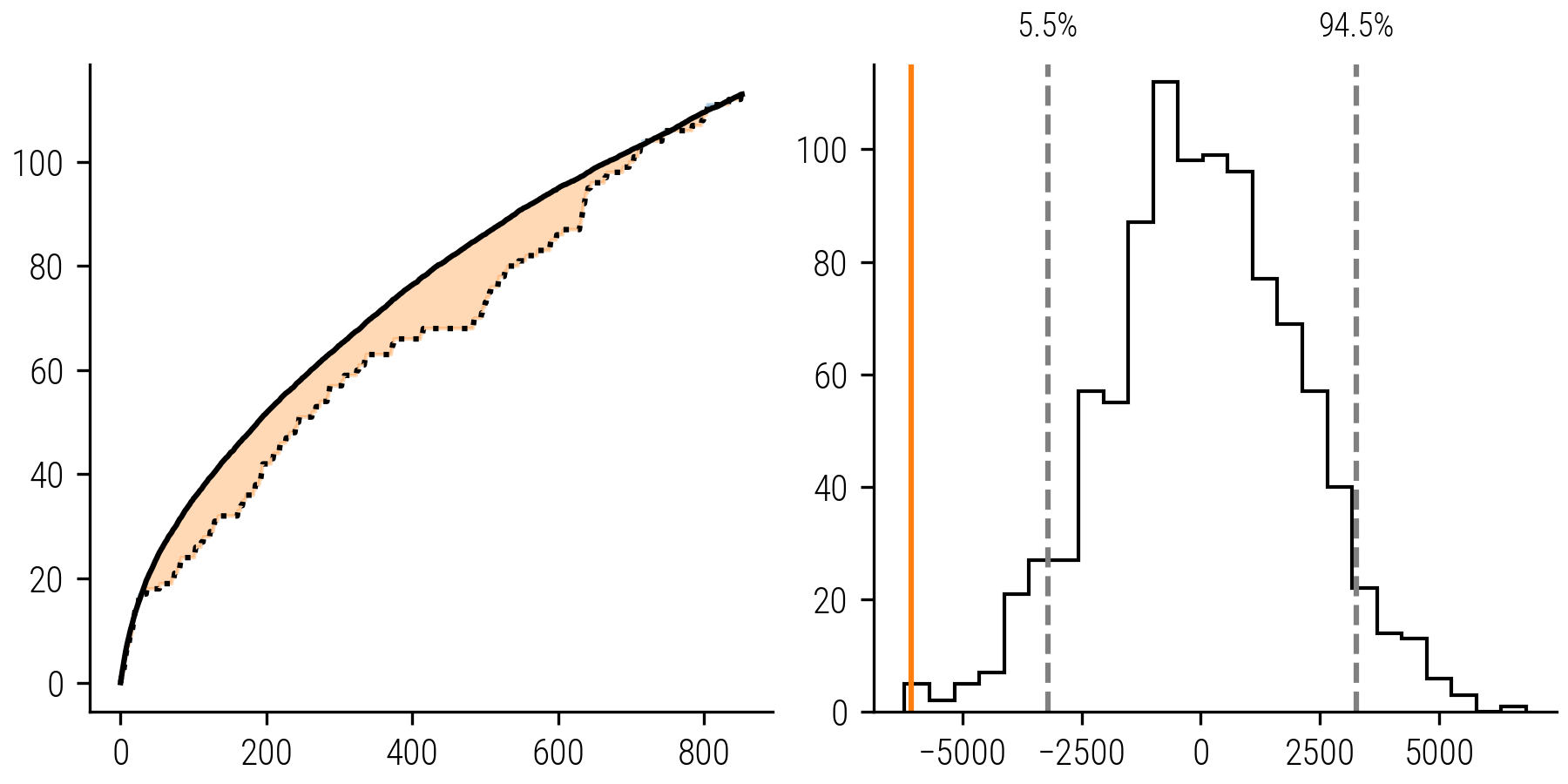
Figure 6: Left: Collector’s curve and corresponding rarefaction curve. Right: Histogram of Bootstrapped AUC Differences: The distribution represents 1000 simulated collectors’ curves compared to the rarefaction curve. The orange vertical line marks the empirical AUC difference, with its position relative to the 89% confidence interval indicating the significance of the collector’s bias.
By examining the position of the empirical difference relative to the bootstrapped distribution, we can infer the likelihood of the observed deviation. Specifically, we assess if the empirical value falls within the 89% confidence interval (the .89 quantile) of the bootstrapped differences. If the empirical value lays outside this range, it suggests that the deviation from the rarefaction curve is indeed significant or – to use a less loaded term – marked and not a product of random variation. This analysis gives more confidence in marking Wever as a conservative collector.
In applying our bootstrapping method to assess the collection biases of six folklorists, the results, as illustrated in the plot below, are quite revealing. The analysis indicates that Jaarsma and Wever’s collections exhibit a marked conservative trend, with their empirical AUC differences falling well outside the expected range of random curves. This suggests a significant preference for familiar story types over novel ones in their folktales collection process.
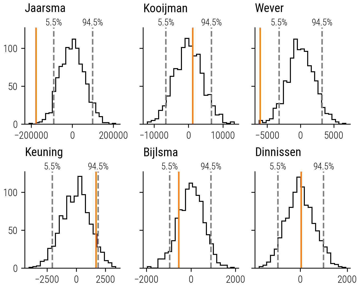
Figure 7: Bootstrapping Analysis of Collector Biases: The histograms represent the distribution of AUC differences for 1000 bootstrapped collector’s curves. The vertical orange lines indicate the empirical AUC differences for each collector.
Keuning’s results, while less pronounced, still indicate a tendency towards exploration. His empirical AUC difference leans towards the upper quantile, suggesting a bias towards collecting new story types.
The remaining collectors – Kooijman, Bijlsma, and Dinnissen – do not show substantial deviations from the mean AUC differences. Their collecting patterns do not significantly differ from what would be anticipated under a neutral model, indicating no strong bias towards either exploration or exploitation in their approach to collecting folktales. This analysis allows us to quantitatively measure and compare the collection strategies of individual collectors.
Adjusting for Shifts in Collection Strategy
The initial analysis simplified the collection behaviors into a single overarching bias for each collector. Yet, as observed in some of the collector’s curves, such as the one depicted for Keuning in Figure 4, collecting is not a static endeavor. Collectors’ approaches evolve, reflecting a dynamic interplay between conservatism and exploration. Keuning’s narrative, for instance, begins with a conservative stance in his early collecting days, gradually transitioning to a more expansive strategy. Recognizing this fluidity, it’s essential to enhance our analytical methods to pinpoint and understand these shifts in biases throughout the collectors’ careers.
The updated method incorporates a segmented approach to analyze the collector’s curve, allowing for a more dynamic assessment of each collector’s inclinations towards familiar or novel story types. This segmentation is determined by analyzing the pointwise differences between the collector’s curve and the corresponding rarefaction curve. A negative difference indicates a bias towards familiar stories, while a positive difference signals a leaning towards new, uncharted types. To ensure meaningful analysis, we focus on segments that maintain a consistent bias for a minimum duration of 20 timesteps.
For each defined segment, we calculate the Area Under the Curve (AUC) for the collector’s curve, the rarefaction curve, and the simulated curves previously generated. We then assess the AUC difference between the empirical data and the rarefaction curve for each segment. Employing the same statistical framework as our initial approach, we determine whether the observed AUC differences fall outside the confidence interval established by the distribution of the bootstrapped curves.
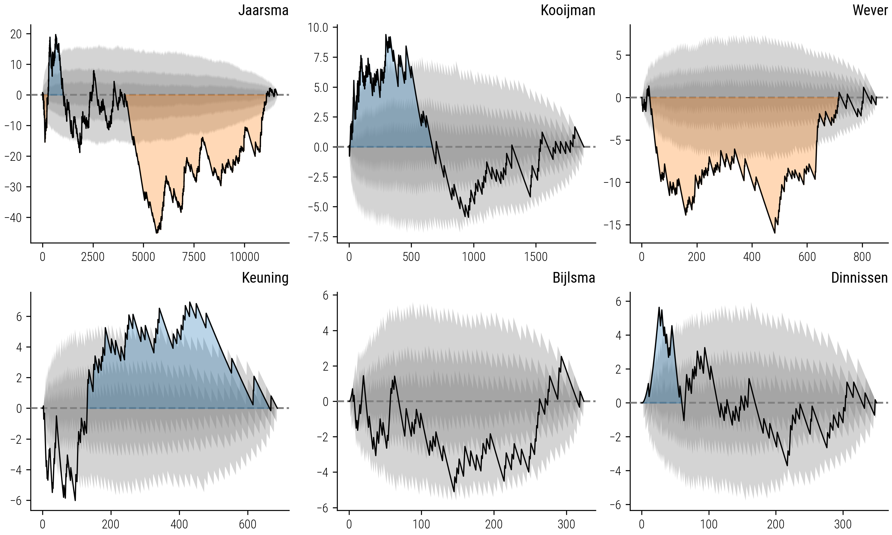
Figure 8: Differential Bias Analysis: The black line represents the pointwise differences between each collector’s curve and the rarefaction curve. Grey areas indicate the confidence intervals from the bootstrapped simulations. Colored areas—blue for exploration bias and orange for familiarity bias—signify periods where the collector’s strategy significantly deviates from the neutral model.
The figure presented here illustrates the nuanced deviations between each collector’s curve and the corresponding rarefaction curve. The shaded grey areas denote the confidence intervals derived from the difference between a thousand simulated curves and the rarefaction curve, representing the expected variance due to chance alone. Where the collector’s curve significantly diverges from the rarefaction curve, we highlight the area to indicate a significant bias: blue for segments showing an exploration bias where collectors favored novel story types, and orange for segments indicating an exploitation or familiarity bias, where collectors tended to prefer stories they had already encountered. This visual representation allows us to discern periods within the collectors' activities where their strategies markedly lean towards exploring new material or exploiting familiar themes, offering a dynamic view of their collecting behaviors over time.
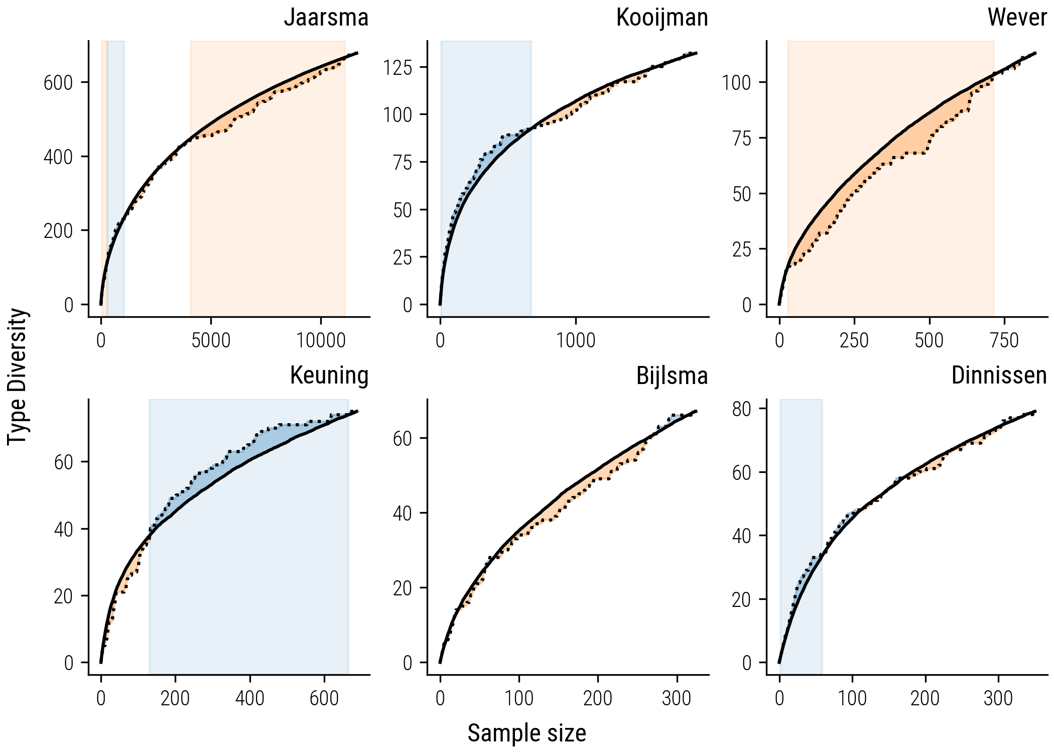
Figure 9: Collector’s Curve Segmentation by Bias: The plots feature the collector’s curves against the rarefaction curves, with significant deviations highlighted. Blue segments indicate a significant exploration bias, while orange segments denote a significant familiarity bias, providing insight into the dynamic collection strategies over time.
The segmentation method enabled us to identify specific intervals where the bias for novelty or familiarity seems less likely random. These intervals are denoted by the colored backgrounds on updated Figure 9 with collector’s curves: a blue backdrop signifies segments where the collector’s curve significantly deviates above the rarefaction curve, indicating periods of exploration bias; conversely, an orange backdrop highlights segments where the collector’s curve falls significantly below, indicating periods of exploitation or familiarity bias.
The refined analysis uncovers more intricate patterns in the collecting behaviors than we previously discerned. For instance, collectors such as Kooijman, Keuning, and Dinnissen displayed more pronounced biases during specific intervals of their collecting activities. Kooijman’s approach, while not consistently biased, began with a marked inclination towards gathering new stories—a trend that was not evident in the overarching analysis. On the contrary, Keuning exhibited an initial preference for familiar tales before shifting to a more exploratory collection strategy, a transition that aligns with our earlier observations. Meanwhile, Bijlsma’s collecting pattern closely mirrors that of the random curves, suggesting a balanced strategy with no discernible bias towards either novelty or familiarity.
Outlook
In the next notebook, I will delve deeper into the functional differences between stories within the folktale collections. While the current analysis employs the traditional folktale type classification to quantify unique stories, some folktale types bear closer resemblance to each other than others. To capture this subtlety, I plan to employ a diversity metric that acknowledges the varying degrees of similarity between folktale types.
This refined approach will hopefully allow us to paint a more nuanced portrait of each collector’s strategy. For instance, a collector might exhibit a broad range in the types of folktales gathered, yet these types could be closely related in theme or structure. Conversely, another collector might focus on a narrower range of folktale types but explore a wide variety of versions within those types.