Motivation
In a recent set of experiments, we aim to use Unseen Species Models such as the Chao1 estimator (see Demystifying Chao1 with Good-Turing) to correct for biases in historical criminology data. Specifically, we aim to estimate the true number of criminals active during a particular year in 19th century Brussels and Antwerp. For these experiments, we rely on police reports, which list the apprensions of individuals at different moments in time. Since the way these data are constructed is in many ways different from registration campaigns done by ecologists, we want to obtain a more mechanistic understanding of how such data could be generated and how this generation process affects the accuracy of Unseen Species Models.
Simulation model
In the simulation model below, we assume that a population of \(N\) criminals is monitored during \(T\) timesteps. At each timestep \(t\), each criminal \(j\) can be observed and successively apprehended with a constant probability \(p\). Apprehended invididuals are the taken out of the population (i.e. put in jail) for \(t\) timesteps, \(t \sim \textrm{Poisson}(\lambda)\), where \(\lambda\) represents the average jail time rate. Naturally, individuals in jail cannot be observed.
import numpy as np

def simulate_population(popsize, p_observe, timesteps, jailrate=0):
    arrests = np.zeros((timesteps, popsize), dtype=int)
    free = np.ones((timesteps, popsize), dtype=int)
    for t in range(timesteps):
        for i in range(popsize):
            arrest = np.random.binomial(1, p_observe * free[t, i])
            arrests[t, i] += arrest
            if arrest and jailrate > 0:
                free[t:t + np.random.poisson(jailrate), i] = 0
    return arrests
We run the simulation for \(T=10\) timesteps, with a true population of \(N=100\) and an apprehension probabililty at each timestep of \(p=0.1\):
arrests = simulate_population(100, 0.1, 10).sum(0)
print(arrests)
[0 0 1 0 2 0 0 1 1 0 2 0 0 0 1 1 0 2 3 1 2 0 0 0 1 1 0 0 1 2 2 0 0 1 0 1 0
 1 1 1 3 0 2 1 1 2 2 0 1 1 3 2 0 2 2 0 3 0 4 2 0 1 0 1 1 4 1 1 1 2 1 1 1 0
 1 0 2 1 1 1 2 0 1 1 2 0 1 2 0 1 0 1 1 1 1 0 0 1 0 0]
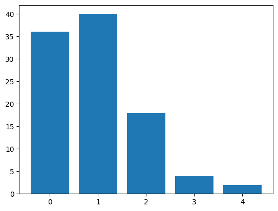
With the apprehension probability set to \(p=0.1\), most individuals are apprehended a single time, and a relatively large fraction has not been observed at all:
import matplotlib.pyplot as plt

plt.bar(list(range(arrests.max() + 1)), np.bincount(arrests));
The goal then is to estimate the size of this missing fraction. For this, we use Chao’s Unseen Species Model “Chao1” (Chao 1984), as implemented in the Python package Copia:
from copia import diversity

int(diversity(arrests, method="chao1"))
107
In this particular case, the Chao1 estimator slightly overestimates the true population size of criminals. In what follows, I try to obtain a more comprehensive understanding of the interplay of the different variables. The goal is to learn more about the conditions under which we can trust the predictions of the different unseen species models.
Results
First, let’s study the effect of the jail time parameter \(\lambda\) in relation to the number of registration moments (i.e., timesteps). The jail time parameter specifies the number of timesteps an individual is taken out of the population once apprehended. The following figure illustrates some settings:
fig, axes = plt.subplots(ncols=4, figsize=(9, 3), layout="constrained")
for i, l in enumerate((1, 2, 5, 10)):
    dist = np.random.poisson(l, size=1000)
    axes[i].hist(dist, bins="fd")
    axes[i].set_title(fr"$\lambda_{{\mathrm{{jail}}}} = {l}$")
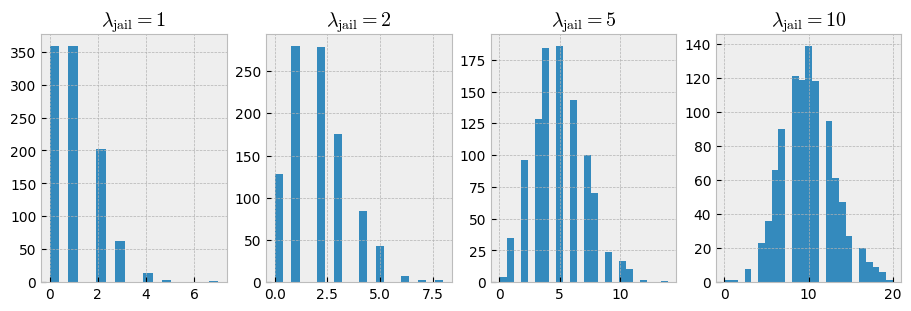
With \(\lambda=1\), jail time is mostly limited to 1 or even 0 timesteps. By contrast, with \(\lambda=5\) or \(\lambda=10\), the mean jail time increases to approximately 5 and 10 timesteps respectively. Let’s study the effect of \(\lambda\) on the estimation accuracy. The code below estimates the true population size for populations generated with \(\lambda \in \{ 0, 1, 2, 5, 8, 10 \}\) and \(T \in \{ 1, 5, 10, 25, 50, 100 \}\). In all experiments, \(N\) is set to 500, and \(p\) to 0.1.
import matplotlib.pyplot as plt
import pandas as pd
plt.style.use("bmh")

fig, axes = plt.subplots(ncols=3, nrows=2, figsize=(9, 6), layout="constrained")
axes = axes.flatten()

N_criminals, p_detect = 500, 0.1
n_timesteps = 1, 5, 10, 25, 50, 100
jailrates = 0, 1, 2, 5, 8, 10

for i, rate in enumerate(jailrates):
    results = []
    for timesteps in n_timesteps:
        for _ in range(100):
            pop = simulate_population(N_criminals, p_detect,
                                      timesteps, jailrate=rate).sum(0)
            try:
                estimate = diversity(pop, method="chao1")
            except ValueError:
                estimate = 0
            results.append({"timesteps": timesteps, "estimate": estimate})

    df = pd.DataFrame(results)
    df.plot.box(by="timesteps", ax=axes[i])
    axes[i].set_title(fr"$\lambda_{{\mathrm{{jail}}}} = {rate}$")
    axes[i].axhline(N_criminals, ls="--", color="C1")
    axes[i].set_yscale("log")

fig.supxlabel("# registration moments (e.g. days)")
fig.supylabel("Estimated population size");
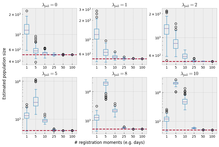
With only a single registration moment – which would be the equivalent of a single day in the police reports – the model seems to consistently overestimate the true poopulation size. Additionaly, removing arrested individuals from the population affects the accuracy of the estimator negatively, up until \(T=25\). However, it is misleading to conclude that a sufficient number of registration moments solves our issues. With the combination of \(T \ge 25\) and \(p = 0.1\), almost the entire population has been observed at least once. The following plot makes that more clear:
fig, axes = plt.subplots(ncols=3, nrows=2, figsize=(9, 6), constrained_layout=True)
axes = axes.flatten()

for i, rate in enumerate(jailrates):
    results = []
    for timesteps in n_timesteps:
        for _ in range(100):
            pop = simulate_population(N_criminals, p_detect, timesteps, jailrate=rate).sum(0)
            results.append({"timesteps": timesteps, "estimate": (pop > 0).sum() / N_criminals})

    df = pd.DataFrame(results)
    df.plot.box(by="timesteps", ax=axes[i])
    axes[i].set_title(fr"$\lambda_{{\mathrm{{jail}}}} = {rate}$")

fig.supxlabel("# registration moments (e.g. days)")
fig.supylabel("Fraction observed population");
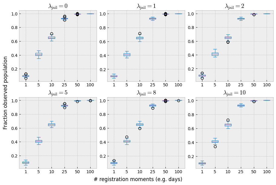
The probability of observation thus interacts with the number of registration moments as well as with the jail time parameter \(\lambda\). The plot below studies this relationship in a bit more detail. Here we investigate different values of \(p\), ($p ∈ \{0.001, 0.01, 0.1, 0.5 \}), combined with an increasing number of registrations:
fig, axes = plt.subplots(ncols=3, nrows=2, figsize=(9, 6), layout="constrained")
axes = axes.flatten()
apprehension_probabilities = 0.001, 0.01, 0.1, 0.5

for i, timesteps in enumerate(n_timesteps):
    results = []
    for j, p_detect in enumerate(apprehension_probabilities):
        for _ in range(100):
            pop = simulate_population(N_criminals, p_detect, timesteps, jailrate=2).sum(0)
            try:
                estimate = diversity(pop, method="chao1")
            except ValueError:
                estimate = 0
            results.append({"p_detect": p_detect, "estimate": estimate})

    df = pd.DataFrame(results)
    df.plot.box(by="p_detect", ax=axes[i])
    axes[i].set_title(f"# registrations = {timesteps}")
    axes[i].axhline(N_criminals, ls="--", color="C1")
    axes[i].set_yscale("log")

fig.supxlabel("probability of apprehension")
fig.supylabel("Estimated population size");
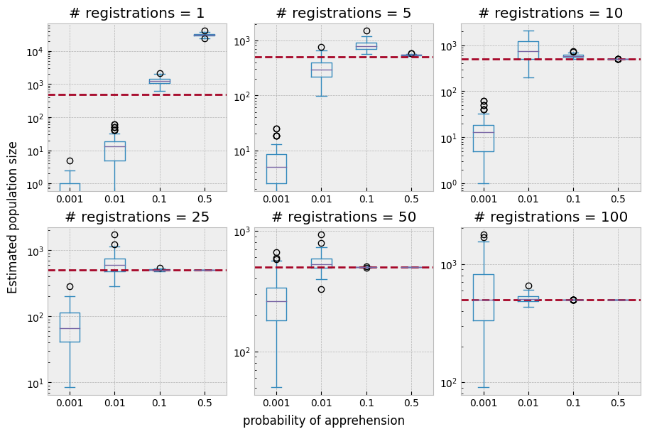
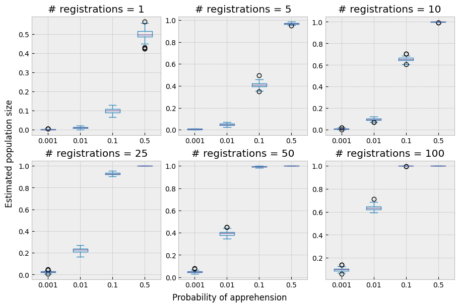
Finaly, the relationship between detection probability and registration moments in terms of poulation coverage becomes more clear from the following plot:
fig, axes = plt.subplots(ncols=3, nrows=2, figsize=(9, 6), layout="constrained")
axes = axes.flatten()
apprehension_probabilities = 0.001, 0.01, 0.1, 0.5

for i, timesteps in enumerate(n_timesteps):
    results = []
    for j, p_detect in enumerate(apprehension_probabilities):
        for _ in range(100):
            pop = simulate_population(N_criminals, p_detect, timesteps, jailrate=2).sum(0)
            results.append({"p_detect": p_detect, "estimate": (pop > 0).sum() / N_criminals})

    df = pd.DataFrame(results)
    df.plot.box(by="p_detect", ax=axes[i])
    axes[i].set_title(f"# registrations = {timesteps}")

fig.supxlabel("Probability of apprehension")
fig.supylabel("Estimated population size");