Functional Diversity
In some previous notebooks (see, for example, here, here, and here), I have discussed the concept of cultural diversity and how methods from ecology can be used to estimate the lower bound of unseen cultural diversity. In these notebooks, diversity was understood simply as the number of unique items in a collection (e.g., species, narratives, pictures, melodies, etc.), with all elements being considered as equidistant, or, in other words, categorically different. Of course, it only rarely, if ever, happens that all items are exactly equally different from each other. It is much more likely that some species are more similar than others. And the same is true of cultural artefacts.
Imagine two populations “A” and “B”, each consisting of 100 unique items. In terms of categorical diversity, both populations have a diversity index of 100. We can, however, also describe each item in terms of certain characteristics and properties, as shown below, in which the items are represented as points in a two-dimensional space (representing weight and height, for example):
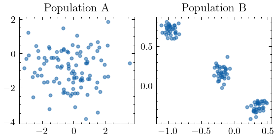
Clearly, the items in population B can grouped into three clusters, whereas there does not appear to be any clustering structure in population A, and as a whole the distance between all individual items seems larger in population A than in B. In short, if we treat diversity as a scalar phenomenon rather than a categorical one and thus incorporate similarities between items in our definition of diversity, it is clear that population A is more diverse than population B.
In ecology, several diversity measures have been developed that account for differences between species and individuals. Most of these measures attempt to estimate functional diversity in terms of the similarities between certain attributes. Based on these attributes, then, we can compute pairwise distances between species using well-known distance metrics (such as the “Euclidean distance” or “Jaccard dissimilarity index”). “Functional Attribute Diversity” (FAD) (Walker, Kinzig, and Langridge 1999), is an example of such a measure that expresses functional diversity as the sum of the pairwise distances between species:
\[ \textrm{FAD} = \sum^S_{i = 1} \sum^S_{j = 1} d_{ij} \]
Here, \(S\) represents the number of unique species, and \(d_{ij}\) the distance between species \(i\) and \(j\).
Functional Diversity in the Dutch Folktale Database
To get a feel for the FAD measure compared to other more common measures such as “richness” (i.e., the number of unique elements), I apply the measure to a collection of Dutch folktales from the Dutch Folktale Database (also see Estimating Unseen Shared Cultural Diversity). Many stories in the database have been categorised according to the Aarne-Thompson-Uther index (Uther 2004), which is an international index for categorising folktales. This index distinguishes numerous different folktale types, that are defined on the basis of a set of motifs that often occur in instantiations these types. Each story type in the index provides a short summary of the most common plot developments along with a sequence of motifs from Thompson’s Motif Index. An example of such a description reads as follows:
ATU 327A, Hansel and Gretel. A (poor) father (persuaded by the stepmother) abandons his children (a boy and a girl) in the forest [S321, S143]. Twice the children find their way back home, following scattered pebbles [R135]. On the third night, birds eat the scattered peas (bread-crumbs) [R135.1]. The children come upon a gingerbread house which belongs to a witch (ogress) [G401, F771.1.10, G412.1]. She takes them into her house. The boy is fattened [G82], while the girl must do house-work. The witch asks the boy to show his finger in order to test how fat he is [G82.1], but he shows her a bone(stick) [G82.1.1]. When the witch wants to cook the boy, the sister deceives her by feigning ignorance and pushes her into the oven [G526, G512.3.2]. [. . . ] The children escape, carrying the witch’s treasure with them. Birds and beasts(angels) help them across water. They return home.
This example shows that the tale type ATU 327A contains twelve motifs, such as S321 Destitute parents abandon children, G401 Children wander into ogre’s house, G82.1 Cannibal cuts captive’s finger to test fatness, and G526 Ogre deceived by feigned ignorance of hero.
Below, I will use use these motif sequences to compute the distances between stories, and subsequently, the FAD of the folktale collection. We start with loading the data:
dfd = pd.read_csv("data/dfd-motifs.csv")
dfd.head()
| count | storytype | motifs | category | |
|---|---|---|---|---|
| 0 | 2 | ATU 1 | K371.1 | Animal Tales |
| 1 | 7 | ATU 2 | K1021 | Animal Tales |
| 2 | 1 | ATU 2A | K1021.1 | Animal Tales |
| 3 | 2 | ATU 15 | K372 | Animal Tales |
| 4 | 1 | ATU 20C | Z43.3 | Animal Tales |
An rudimentary yet important measure of diversity is the number of unique items or “richness” in an assemblage or collection. The richness of the folktale collection is simply the number of unique story types:
dfd['storytype'].nunique()
348
Similarly, we can compute this richness per folktale type category. The index defines seven categories (Tales of Magic I and II are essentially one category) with the following richness diversity:
dfd["category"].value_counts()
Let us now compute the Functional Attribute Diversity of the folktale collection as a whole and per category. As our distance measure, we will compute the Jaccard dissimilarity index, which is a set-based dissimilarity measure:
import itertools

def jaccard_distance(a, b):
    return 1 - len(a.intersection(b)) / len(a.union(b))

FAD = 0
motifs = dfd["motifs"].str.split(";").apply(set).values
for a, b in itertools.combinations(motifs, 2):
     d = jaccard_distance(a, b)
     assert d <= 1
     FAD += d * 2

print(f"FAD = {round(FAD)}")
FAD = 131374
By themselves, these numbers are rather difficult to interpret. I’m not quite sure how to interpret the value of 131374. It becomes more interesting and interpretable when we compare the FAD of different categories. So, let’s do that and compute the FAD of the seven categories and compare their diversity measures:
FADs = {}
for category in df["category"].unique():
    FAD = 0
    motifs = dfd.loc[dfd["category"] == category, "motifs"].str.split(";").apply(set).values
    for a, b in itertools.combinations(motifs, 2):
         d = jaccard_distance(a, b)
         FAD += d * 2
    FADs[category] = FAD

for category in sorted(FADs, key=FADs.get, reverse=True):
    print(category, round(FADs[category]))
Anecdotes and Jokes 19736
Animal Tales 4966
Tales of Magic I 2548
Tales of Magic II 866
Realistic Tales 812
Religious Tales 450
Tales of the Stupid Ogre 240
Formula Tales 6
The FAD measure shows more pronounced differences between the categories. For example, when “Anecdotes and Jokes” has about twice the number of unique stories than “Animal Tales”. This difference becomes even larger for the FAD, for which Anecdotes and Jokes has a FAD that is \(\frac{19736}{4966} \approx 4\) times larger than that of Animal Tales.
Unseen Functional Diversity
The ATU index is a collection of all defined story types. However, in actual folktales collections, we rarely encounter all of these types, as they often represent incomplete samples, offering only limited insight into the potential diversity of folktales. The same problem arises in ecology. When bioregistration campaigns are used to measure categorical or functional diversity in a given area, there is always a chance that not all species and therefore not thee full feature space had been observed. Can we somehow correct the bias introduced by this by estimating how much functional diversity is unobserved?
Chao et al. (2017) propose an estimator of undetected fuctional diversity to correct for this bias. Their method is based on the Good-Turing framework I discussed in Demystifying Chao1 with Good-Turing. The method estimates a lower-bound of the unseen FAD in way comparable to the estimation of the number of unseen species shared between two assemlages (see Estimating Unseen Shared Cultural Diversity). (Chao et al. 2017) show that the a lower-bound of the true FAD can be expressed as the sum of the following four terms:
\[ \textrm{FAD} = \textrm{FAD}_{\textrm{obs}} + \textrm{F}_{0+} + \textrm{F}_{+0} + \textrm{F}_{00}. \]
Here, \(\textrm{FAD}_{\textrm{obs}}\) represents the FAD of the observed sample. \(F_{0+}\) and \(F_{+0}\) represent the unseen FAD of pairs of items in which one item is missing from the sample. Finally, \(F_{00}\) represents the FAD for items that are both missing from the sample.
Just as I explained before in Demystifying Chao1 with Good-Turing and Estimating Unseen Shared Cultural Diversity, we aim to compute the mean distance \(\theta_{rr}\) of any two pair of items (or species) that occur exactly \(r\) times. To do that, (Chao et al. 2017) propose the estimator \(\theta_{rr}\):
\[ \hat{\theta}_{rr} = \frac{(r + 1)^2 F_{r + 1, r + 1}}{(n - 2r)(n - 2r - 1)F_{rr}}, r = 0, 1, 2, \ldots \]
Unfortunately, we do not know \(F_{00}\) nor do we know about \(\theta_{00}\). We do know, however, that \(\frac{F_{11}}{n}\) is a good estimate of the product of \(\theta_{00}\) and \(F_{00}\). And like with the Good-Turing derivation of Chao1, it should intuitively hold that \(\theta_{00} \leq \theta_{11}\). And if that is the case we can compute a lower bound for \(F_{00}\) with:
\begin{align*} F_{00} = \frac{\theta_{00} F_{00}}{\theta_{00}} \geq \frac{\theta_{00} F_{00}}{\theta_{11}} & = \frac{\frac{F_{11}}{n(n - 1)}}{\frac{4F_{22}}{(n - 2)(n - 3)F_{11}}} \\ & = \frac{(n - 2)}{n} \frac{(n - 3)}{(n - 1)} \frac{F^2_{11}}{4F_{22}} \end{align*}
For \(F_{0+}\) and \(F_{+0}\), we apply the same strategy as explained in Estimating Unseen Shared Cultural Diversity, which gives us the following expression to compute a lower-bound for the true functional diversity in an assemblage:
\[ \textrm{FAD}_{\textrm{Chao1}} = \textrm{FAD}_{\textrm{obs}} + \frac{(n - 1)}{n} \frac{F^2_{1+}}{2F_{2+}} + \frac{(n - 1)}{n} \frac{F^2_{+1}}{2F_{+2}} + \frac{(n - 2)}{n} \frac{(n - 3)}{(n - 1)} \frac{F^2_{11}}{4F_{22}} \]
Unseen Functional Diversity in the Dutch Folktale Database
To conclude this notebook, let us apply the \(\textrm{FAD}_{\textrm{Chao1}}\) to the folktale database to estimate its unseen functional diversity. We start by implementing the FAD estimator in the following lines of code:
def compute_fad_chao1(dm, counts):

    FAD_obs = np.sum(dm[counts > 0][:, counts > 0])
    mean_distance = np.mean(dm)
    F1p = np.sum(dm[counts == 1][:, counts >= 1])
    Fp1 = np.sum(dm[counts >= 1][:, counts == 1])
    F2p = np.sum(dm[counts == 2][:, counts >= 1])
    F2p = max(F2p, mean_distance)
    Fp2 = np.sum(dm[counts >= 1][:, counts == 2])
    Fp2 = max(Fp2, mean_distance)
    F11 = np.sum(dm[counts == 1][:, counts == 1])
    F22 = np.sum(dm[counts == 2][:, counts == 2])
    F22 = max(F22, mean_distance)
    assert round(F1p) == round(Fp1), (F1p, Fp1)
    assert round(F2p) == round(Fp2), (F2p, Fp2)
    n = sum(counts)
    k = (n - 1) / n
    F0p = k * (F1p ** 2) / (2 * F2p)
    Fp0 = k * (Fp1 ** 2) / (2 * Fp2)
    F00 = ((n - 2) / n) * ((n - 3) / (n - 1)) * ((F11 ** 2) / (4 * F22))
    return {
        "obs": round(FAD_obs),
        "F0+": round(F0p),
        "F+0": round(Fp0),
        "F00": round(F00),
        "FAD": round(FAD_obs + F0p + Fp0 + F00)
    }
Next, we implement the following wrapper function, which makes it slightly more convenient to compute the FAD for different folktale categories:
def estimate_fad(df, category=None):
    if category is not None:
        df = df.loc[df["category"] == category]
    counts = df["count"].values
    motifs = df["motifs"].str.split(";").apply(set).values
    V = counts.shape[0]
    dm = np.zeros((V, V))
    for i in range(V):
        for j in range(V):
            dm[i, j] = dm[j, i] = jaccard_distance(motifs[i], motifs[j])
    return compute_fad_chao1(dm, counts)
Let us first apply the estimator to the complete collection. Below, I compute the FAD as well as the ratio between the observed FAD and the estimated lower-bound of the true FAD:
fad = estimate_fad(dfd)
print(f"Observed FAD: {fad['obs']}, Estimated FAD: {fad['FAD']}, FAD coverage: {fad['obs'] / fad['FAD']:.2f}")
Observed FAD: 131374, Estimated FAD: 287015, FAD coverage: 0.46
We estimate a FAD of 287015, of which 46% is already available in the folktale database. This means that still a considerate amount of variation is not yet part of the database. It is also to be expected that the FAD coverage varies by story category. Therefore, I calculate the FAD again below for each folktale category, in order to identify any differences:
for category in dfd["category"].unique():
    fad = estimate_fad(dfd, category)
    print(category, f"coverage: {fad['obs'] / fad['FAD']:.2f}")
Animal Tales coverage: 0.39
Tales of Magic I coverage: 0.24
Tales of Magic II coverage: 0.46
Religious Tales coverage: 0.54
Realistic Tales coverage: 0.43
Tales of the Stupid Ogre coverage: 0.36
Anecdotes and Jokes coverage: 0.58
Formula Tales coverage: 0.50
These number show that the functional diversity in “Anecdotes and Jokes” is relatively well covered by the folktale database, while “Tales of Magic I” (24%) and “Animal Tales” (39%) have a much lower diversity coverage.